From an Economic Question to a Local Projection

Lecture 01

These notes pair with the slides, the Shock-to-Response Explorer browser lab, and Practicum 01. The PDF version, compiled from the same source, is under “Other Formats.”

In late June 1950, North Korean forces crossed into South Korea. Within weeks, American newspapers and business magazines were reporting plans for a large and lasting rise in military spending. Ramey’s narrative series prices such reports as the change in the expected present value¹ of government spending (Ramey, 2011). For the third quarter of 1950 it records news worth 179.4 billion dollars, which is 0.600 of the previous quarter’s nominal trend GDP² at an annual rate (Ramey and Zubairy, 2018). A policymaker reading those reports would want to know what the buildup would do to output over the next three years.

The path that followed is easy to read. Real GDP stood 2.75 percent below trend in 1950Q2 and 5.12 percent above it in 1953Q1, ten quarters after the news arrived: a rise of 7.87 points of trend GDP. It is tempting to call those 7.87 points the effect of the news. Many other things happened in the same quarters, though. Taxes rose; in the postwar tax record assembled by Romer and Romer (2010), the largest increases motivated by spending came during the Korean War. The March 1951 Treasury–Federal Reserve Accord³ freed monetary policy. Wage and price controls were imposed in January 1951 and dismantled early in 1953 (Rockoff, 1984). The rise of 7.87 points mixes the news with all of these.

So the question is not what happened next. It is what happened because of the news, and answering it requires a path nobody observed: the one GDP would have followed had the news not arrived, with everything else as it was. This lecture turns that comparison into a regression. We start in an economy small enough that the unobserved path can be computed exactly and derive a regression whose coefficient recovers the comparison there. Then we build that regression’s rows by hand and return to the quarterly data with one estimated response and a list of what it has not yet earned.

By the end of the lecture, you should be able to:

1. define the causal response at horizon h as the gap between the realized path and the path without the intervention, and distinguish it from the change since the date before the intervention;
2. iterate y_t=\rho y_{t-1}+\theta_0 s_t+v_t forward to derive \theta_h=\theta_0\rho^h, and show that the horizon-h regression of y_{t+h} on a constant, s_t, and y_{t-1} has \beta_h=\theta_h, \gamma_h=\rho^{h+1}, and a residual built from disturbances dated t through t+h and shocks dated t+1 through t+h;
3. build the regression rows for h=0,1,2 by hand, state T_h=T-h-p, and compute \hat\beta_h from those rows;
4. estimate \hat\beta_h for h=0,\dots,H in a Stata loop that stores \hat\beta_h and T_h, and draw a response graph whose caption names the intervention, the units, and the counterfactual; and
5. explain what one estimated coefficient measures and where its variation comes from, why a single episode cannot identify it, and which claims a first data application has not yet earned.

The lecture assumes ordinary least squares (the slope as a covariance over a variance, and the slope on a 0–1 regressor as a difference in means), expectation and independence, and elementary Stata: tsset, time-series operators, loops, regress, and stored results. No time-series course is assumed; the one autoregression we need is built from scratch and iterated by hand. Standard errors, instruments, and vector autoregressions come later.

1 The Question: An Intervention, an Outcome, and a Path We Never See

The Korean episode has three parts that recur in every problem of this course. Something happens at a date: news arrives, a policy rate moves, a state changes its banking law. An outcome is measured at that date and afterwards. And the question compares that outcome with what it would otherwise have been. The first two parts can be measured. The third cannot, and an economy small enough to compute by hand shows why no single observed path supplies it.

1.1 Intervention, Outcome, and Two Paths

Write s_t for the intervention variable dated t and y_t for the outcome. In the opening, s_t is a quarter’s military news measured as a fraction of trend GDP, and y_t is real GDP divided by trend GDP. The name is deliberately neutral. Calling s_t a shock would claim that nothing else systematically moves with it, and that claim needs an argument, which Lecture 3 supplies. Until then s_t is simply the variable whose effect we want.

The data record one sequence of outcomes, the realized path. It carries the effect of s_t together with the effect of every other disturbance that arrived before and after. The counterfactual path, written y^{c}_t, is the sequence the same economy would have produced without the intervention at date t and with every other disturbance exactly as it was. The superscript c marks counterfactual objects throughout the course. Nobody observes y^{c}_t.

The causal response h periods after the intervention is the gap between the two paths at the same date:

\theta_h=y_{t+h}-y^{c}_{t+h}. \tag{1}

Read Equation 1 across, not down the calendar. Both terms are dated t+h, so the equation compares two versions of one period, not one period with an earlier one. The units of \theta_h are the units of y; when the intervention is a one-unit change in s_t, they are units of y per unit of s. In the Korean example the gap would be measured in points of trend GDP. The response carries no date subscript here because, in the economies of this lecture, the gap does not depend on when the intervention arrives; Section 2 and Section 3 show why. This is the sense in which Stock and Watson (2018) define dynamic causal effects in macroeconomics: a comparison of the outcomes that would follow different values of the intervention, not a description of what followed the one value that occurred.

1.2 The Change Since the Date Before

The number the opening read off the data was a different object: the change in the realized path since the period before the news, y_{t+h}-y_{t-1}. To see how it relates to \theta_h, add and subtract y^{c}_{t+h}:

y_{t+h}-y_{t-1} =\underbrace{\bigl(y_{t+h}-y^{c}_{t+h}\bigr)}_{\theta_h} +\underbrace{\bigl(y^{c}_{t+h}-y_{t-1}\bigr)}_{\text{change without the intervention}}. \tag{2}

The first bracket is the causal response. The second is the change the economy would have made anyway, driven by everything except the intervention. The left side of Equation 2 equals \theta_h only when the second bracket is zero, that is, only when the counterfactual path would have stayed at its pre-intervention level. Nothing guarantees that. A wartime economy with rising taxes, a newly independent central bank, and price controls had many reasons to move.

The decomposition relies on one fact about timing. An intervention at t cannot change y_{t-1}, so the realized and counterfactual paths coincide before t and the same y_{t-1} appears in both brackets. If people act on news before it is recorded, that fact fails; Lecture 3 treats the consequences under the name of anticipation.

1.3 A Twelve-Period Economy Where the Counterfactual Is Known

To watch the two objects diverge with actual numbers, we need an economy in which the counterfactual can be computed. Take twelve periods and the rule

y_t=0.5\,y_{t-1}+s_t+v_t,\qquad t=1,\dots,12,\qquad y_0=0.

Each period’s outcome is half of the previous outcome, plus the intervention, plus a disturbance⁴ v_t that stands for everything else. The intervention is binary: s_t=1 in a period when it occurs and 0 otherwise. Both inputs were drawn once in Stata with seed⁵ 1. Each v_t is a standard normal draw rounded to one decimal, and each s_t is an independent draw equal to one with probability 0.3. The interventions happen to fall at t=1,5,10,12. Section 3 returns to this rule with general coefficients; here it only has to generate numbers.

Table 1 lists the draws and the realized path. To build the counterfactual for the intervention at t=5, set s_5=0, hold every v_t at its drawn value, and run the rule again.

Table 1: The twelve-period economy. The counterfactual y^{c}_t removes only the intervention at t=5 and keeps every v_t. Outcome columns are displayed to four decimals with ties rounded away from zero; the gap column is exact, and every calculation in the notes uses exact values.

t	s_t	v_t	y_t	y^{c}_t	y_t-y^{c}_t	y_t-y_4
1	1	0.9	1.9000	1.9000	0	—
2	0	0.5	1.4500	1.4500	0	—
3	0	0.6	1.3250	1.3250	0	—
4	0	−0.6	0.0625	0.0625	0	0.0000
5	1	−1.7	−0.6688	−1.6688	1	−0.7313
6	0	0.2	−0.1344	−0.6344	0.5	−0.1969
7	0	2.1	2.0328	1.7828	0.25	1.9703
8	0	−1.3	−0.2836	−0.4086	0.125	−0.3461
9	0	0.8	0.6582	0.5957	0.0625	0.5957
10	1	0.6	1.9291	1.8979	0.03125	1.8666
11	0	−0.9	0.0646	0.0489	0.015625	0.0021
12	1	1.5	2.5323	2.5245	0.0078125	2.4698

Before period 5 the two paths are identical, as the timing argument requires. At t=5 the realized outcome is y_5=0.5(0.0625)+1-1.7=-0.66875, while the counterfactual is y^{c}_5=0.5(0.0625)+0-1.7=-1.66875. The gap is exactly one: the intervention added one unit. Yet the realized outcome fell by 0.73125 from y_4=0.0625, because a disturbance of -1.7 arrived in the same period.

From then on the gap halves every period. At t=6 both paths carry forward half of their own previous value and receive the same v_6=0.2, so the only difference left is half of the previous gap, 0.5\times1=0.5. At t=7 the gap is 0.25 and at t=8 it is 0.125. The change since t=4 behaves erratically by comparison: -0.196875, then 1.9703125, then -0.34609375. Figure 1 shows both comparisons.

Figure 1: Two paths, one gap. The causal response to the t=5 intervention is the vertical distance between the realized and counterfactual paths at the same date: 1, 0.5, 0.25, and 0.125 at t=5,\dots,8. The change from the pre-intervention value y_4 is a different quantity, -0.731 at t=5 and 1.970 at t=7, because it also contains every disturbance that arrived after t=4.

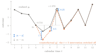
Equation 2 accounts for the difference exactly. At t=7 the realized change of 1.9703125 splits into the causal response 0.25 and a counterfactual change y^{c}_7-y_4=1.7828125-0.0625=1.7203125, which the disturbance v_7=2.1 more than accounts for. Reading the realized change as the effect would overstate the effect nearly eightfold at t=7 and get its sign wrong at t=5. Exercise 1 rebuilds the counterfactual path by hand.

Two features of the example will be needed again. First, the gaps 1, 0.5, 0.25, 0.125 do not depend on any v_t. Change the disturbances and the realized path moves, but the gap sequence does not. Second, the gaps were computable only because we knew the rule and every disturbance. With real data neither is available, so the counterfactual has to be reconstructed from other information. The rest of the lecture is about how a regression does that, and about what it has to assume.

A regression will not switch off one intervention; it pools many. Pooling forces a choice that the table could avoid: how to date a gap.

2 Two Clocks

A statement such as “the response at t=7 is 0.25” hides that choice. It could be a fact about period 7, or a fact about what happens two periods after an intervention. In the twelve-period economy the readings coincide because only one intervention was switched off. They separate as soon as a second intervention is considered.

2.1 Calendar Time and Horizon

Calendar time t is the date of an observation: a quarter such as 1950Q3, or a period in a simulation. In this course it also dates the intervention and, later, the regression row built around it. The horizon h counts the periods after the intervention at which the outcome is measured, so y_{t+h} is read “the outcome h periods after date t.” The horizon is measured in the data’s own periods: quarters in the Ramey–Zubairy data and abstract periods in the simulations. The opening’s 1953Q1 is horizon 10 for news dated 1950Q3.

The response at h=0 is the impact response, the effect within the period of the intervention. In the twelve-period economy it is the gap of 1 at t=5. Horizons count upward to a largest horizon H chosen by the researcher: H=2 for the hand calculations of Section 6, H=12 for the simulations, and H=20 quarters for the military-news data.

Now switch off the intervention at t=10 instead of the one at t=5, again holding every v_t fixed. The gaps at t=10,11,12 are 1, 0.5, and 0.25. On the calendar these are new numbers at new dates. On the horizon clock they are the same numbers as before: 1 at h=0, 0.5 at h=1, 0.25 at h=2. The rule treats an intervention the same way whenever it arrives, so the gap depends on the horizon and not on the date. That property is what allows a single sequence \theta_0,\theta_1,\dots to describe the response to every intervention in a sample. It is an assumption about the economy, stated formally as A1 below; if the effect of news depended on the state of the economy, the response would carry a date as well, which is the subject of Lecture 9.

2.2 The Impulse-Response Function

The sequence of causal responses read as a function of the horizon,

h\longmapsto\theta_h,\qquad h=0,1,\dots,H,

is the impulse-response function. It answers “how does the effect evolve after the intervention?” with a curve rather than a number. In the twelve-period economy the curve starts at 1 and halves each period.

The two clocks sort the objects of this course into two kinds. The realized path of GDP after 1950Q3 is a function of calendar time and belongs to one episode. The impulse-response function is a function of horizon and describes what an intervention does whenever it happens. The rise of 7.87 points was a calendar-time fact about 1950–1953. The policymaker’s question was a horizon-time question.

The distinction has a practical consequence. A regression that estimates the response at one horizon returns one number, so it estimates one point on the curve. Drawing the whole curve takes one estimate per horizon, and each estimate uses its own rows of data, a fact that Section 6 makes concrete. Before estimating anything, though, we need to know what the curve looks like in an economy where it can be derived rather than simulated.

3 The Smallest Model

The twelve-period economy produced a gap that halved every period and ignored the disturbances. Neither fact was an accident of the draws. Both follow from the rule, and seeing why requires writing the rule with general coefficients. The model we use is the smallest one in which an intervention has a response that unfolds over time and in which that response can be derived exactly.

3.1 An Autoregression with an Observed Shock

Let the outcome follow

y_t=\rho\,y_{t-1}+\theta_0 s_t+v_t . \tag{3}

Read Equation 3 from left to right as a recipe for this period’s outcome: carry forward the fraction \rho of last period’s outcome, add \theta_0 units for each unit of the intervention, and add the disturbance v_t. A series that equals a linear function of its own past plus new disturbances is an autoregressive process; this one is first order, written AR(1), because a single lag of y appears. The coefficient \rho measures persistence, the share of any deviation of y that survives into the next period, and it has no units. The coefficient \theta_0 is the impact response, in units of y per unit of s. The twelve-period economy is the case \rho=0.5 and \theta_0=1.

The intervention s_t is drawn independently each period with mean zero and standard deviation \sigma_s. The disturbance v_t is drawn the same way, with mean zero and standard deviation \sigma_v measured in units of y. The two sequences are independent of each other. Generated this way, s_t is an observed shock: a variable we measure directly, that cannot be predicted from the past, and that is independent of every other disturbance moving the outcome. In a simulation this holds by construction. For the military-news series it is a claim, and Lecture 3 examines what would make it believable. (The binary intervention of the twelve-period economy has mean 0.3 rather than zero; a nonzero mean changes only the regression intercept, as Section 4 notes.)

The derivations below use four assumptions. Each is stated once here and cited by number where it does its work.

A1 (Linear, time-invariant dynamics). The outcome follows Equation 3 with the same \rho and \theta_0 at every date. Meaning. An intervention of a given size has the same effect whenever it arrives, and the effects of interventions and disturbances add up. Used in. The forward substitution Equation 4, the response formula Equation 5, and the date-free reading of the response in Section 2. Without it. The gap between paths depends on the date, the state of the economy, or the size of the intervention, so no single sequence \theta_h exists; a regression coefficient then averages different responses with weights the researcher did not choose (Lectures 9 and 10). Kind. A modeling convenience in the simulations and an empirical claim in data.

A2 (Unpredictable intervention). The interventions \{s_t\} are independent over time and identically distributed, with mean zero and variance \sigma_s^2>0. Meaning. Nothing in the past, including past interventions, helps forecast today’s intervention, and the intervention actually varies. Used in. The step \mathbb E[s_tu_{t,h}]=0 in Section 4, which needs s_t to be unrelated to the later interventions inside u_{t,h}, and, together with A3, the step \operatorname{Cov}(s_t,y_{t-1})=0, which leaves \beta_h unchanged when the lagged outcome is dropped. Without it. If interventions are serially correlated, s_t forecasts the later interventions in u_{t,h} and its coefficient absorbs their effects along with its own. Lagged interventions among the controls, as in Ramey and Zubairy’s specification, remove the part of s_t that earlier interventions predict, but they cannot stop s_t from forecasting the interventions that follow it. If \sigma_s^2=0 there is no variation to estimate from. Kind. An identifying restriction.

A3 (Independent disturbances). The disturbances \{v_t\} are independent over time and identically distributed, with mean zero and variance \sigma_v^2, and the whole sequence is independent of \{s_t\}. Meaning. Whatever moves the outcome through v_t neither causes nor is caused by the intervention, at any lead or lag. Used in. The steps \mathbb E[s_tv_{t+j}]=0 and \mathbb E[y_{t-1}u_{t,h}]=0 in Section 4. Without it. A disturbance correlated with s_t is a common cause of the intervention and the outcome, and the regression coefficient moves away from \theta_h; Lecture 3 derives the size of that bias. If the disturbances are serially correlated but still independent of the interventions, \beta_h still equals \theta_h, but \gamma_h no longer equals \rho^{h+1}, because y_{t-1} then also forecasts later disturbances. Kind. Independence from the interventions is an identifying restriction; independence over time is a convenience that keeps the control’s coefficient simple.

A4 (Stationarity). |\rho|<1, and the process has run long enough that y_{t-1} has the same distribution at every date. Meaning. Deviations fade, and the averages that define a population regression are the same whichever date we examine. Used in. Treating the regression coefficients of Section 4 as constants rather than functions of t, and the variance \operatorname{Var}(y_t)=(\theta_0^2\sigma_s^2+\sigma_v^2)/(1-\rho^2) used there. Without it. The response formula Equation 5 survives, but with \rho=1 a response never fades and \operatorname{Var}(y_t) grows with t; Lectures 2 and 5 study how estimates and standard errors behave as \rho approaches one. Kind. A mathematical convenience, and in data an empirical claim about persistence.

The twelve-period economy bends A4 slightly, because it starts from y_0=0 rather than from a draw of the long-run distribution. The larger simulations later in the lecture use a burn-in⁶ of 100 periods. For the hand calculations the start is harmless, since two paths that share y_0 have a gap that does not depend on it.

3.2 Iterating Forward

We want the gap at t+h caused by s_t. The model gives y_t in terms of y_{t-1}; substituting it into itself repeatedly expresses y_{t+h} in terms of y_{t-1} and everything that arrives from t onward.

The case h=0 is Equation 3 itself. For h=1, write the rule one period later and replace y_t by Equation 3:

\begin{aligned} y_{t+1}&=\rho\,y_t+\theta_0s_{t+1}+v_{t+1}\\ &=\rho\bigl(\rho\,y_{t-1}+\theta_0s_t+v_t\bigr)+\theta_0s_{t+1}+v_{t+1}\\ &=\rho^2y_{t-1}+\rho\,\theta_0s_t+\rho\,v_t+\theta_0s_{t+1}+v_{t+1}. \end{aligned}

One more substitution gives

y_{t+2}=\rho^3y_{t-1}+\rho^2\theta_0s_t+\rho^2v_t+\rho\,\theta_0s_{t+1} +\rho\,v_{t+1}+\theta_0s_{t+2}+v_{t+2}.

The pattern is visible after two steps. Each substitution multiplies everything already present by \rho and appends the new period’s intervention and disturbance with coefficient one. After h+1 steps,

y_{t+h}=\rho^{h+1}y_{t-1}+\sum_{j=0}^{h}\rho^{h-j}\bigl(\theta_0s_{t+j}+v_{t+j}\bigr). \tag{4}

To confirm Equation 4 at every horizon, argue by induction⁷. It holds at h=0. If it holds at h, then y_{t+h+1}=\rho\,y_{t+h}+\theta_0s_{t+h+1}+v_{t+h+1} multiplies every term of the formula by \rho and appends the j=h+1 term with weight \rho^0=1, which is the formula at h+1.

Equation 4 is an account of where y_{t+h} comes from. The first term is the outcome just before the intervention, discounted by \rho^{h+1} because it has had h+1 periods to fade. The sum collects every intervention and every disturbance dated t through t+h, each discounted by \rho raised to the number of periods it has had to fade. The newest arrivals count fully and the oldest count least.

3.3 The Response Is \theta_0\rho^h

Now run the counterfactual experiment on Equation 4. Remove a one-unit intervention at t, and hold y_{t-1}, every disturbance, and every other intervention fixed. Only the j=0 term of the sum changes, and it changes by \rho^h\theta_0. By the definition Equation 1,

\theta_h=\theta_0\rho^{h}. \tag{5}

The impulse-response function of this economy starts at the impact response \theta_0 and shrinks by the factor \rho each period. Its units are those of \theta_0, units of y per unit of s, at every horizon. Because A1 makes the rule linear, a two-unit intervention has twice this response, and the response does not depend on the date.

Three checks confirm the formula. With \rho=0.5 and \theta_0=1, Equation 5 gives 1, 0.5, 0.25, 0.125, exactly the gaps in Table 1. No disturbance appears in Equation 5, which is why changing the v_t moved the realized path but not the gaps. And the limiting cases do what persistence should: with \rho=0 the response lasts a single period, as \rho approaches one it barely fades, and with \rho<0 it alternates in sign.

Figure 2 isolates the role of persistence. It holds the impact fixed at \theta_0=1 and changes only \rho.

Figure 2: Persistence sets the shape. Both economies have the same impact response, \theta_0=1, and the same size of intervention. With \rho=0.5 the response has fallen to 0.0078 by h=7; with \rho=0.9 it is still 0.478 there. The difference comes entirely from the outcome’s own persistence.

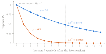
With \rho=0.9 the response first falls below half of its impact value at h=7; with \rho=0.5 it reaches exactly half at h=1 and falls below it at h=2. In this model the intervention contributes only the size of the first step. Everything after that is the outcome’s own dynamics carrying the deviation forward. A central bank’s surprise and a war’s news, if they hit the same outcome with the same impact, would trace the same curve.

That conclusion depends on the single lag. An AR(1) can produce only geometric decay, or an alternating version of it; a response that rises for several periods before it falls, a hump, needs richer dynamics. The military-news response in Section 9 has exactly such a hump. A method that required the researcher to write down the correct dynamics before estimating anything would be fragile for that reason, and the regression derived next does not require it.

The derivation also used two things that data never provide: the rule itself, and the freedom to hold every other term fixed while changing s_t. Data provide rows of (s_t,y_{t-1},y_{t+h}). But Equation 4 already writes y_{t+h} as a coefficient times y_{t-1}, plus a coefficient times s_t, plus everything else.

4 From the Model to a Regression

In the twelve-period economy we found \theta_h by rerunning the rule with one intervention removed. A researcher with data cannot rerun anything. The move available instead is to collect those rows for many dates t and regress the later outcome on the intervention and the earlier outcome. In the economy of Equation 3 that regression recovers \theta_h exactly in population. The work lies in finding which step makes that true.

4.1 Estimands and Population Projections

Three objects need separate names. The estimand is the population quantity a procedure is meant to recover, fixed before any data are drawn; here the causal estimand is \theta_h. A regression targets a population coefficient of its own, defined next, which may or may not equal the estimand. An estimate is a number computed from one sample, and it differs from the coefficient it targets by an amount that changes from sample to sample. The notation keeps population objects and estimates apart: population objects carry no hat, and estimates do.

The population object a regression estimates is a population projection. For an outcome and a set of regressors that includes a constant, it is the linear combination of the regressors with the smallest expected squared prediction error, the best linear predictor⁸. For the outcome y_{t+h} and the regressors (1,s_t,y_{t-1}) it is written

y_{t+h}=\mu_h+\beta_h s_t+\gamma_h y_{t-1}+u_{t,h}, \qquad \mathbb E[u_{t,h}]=\mathbb E[s_tu_{t,h}]=\mathbb E[y_{t-1}u_{t,h}]=0. \tag{6}

The display has two parts. The first equation splits y_{t+h} into a part explained linearly by the regressors and a residual u_{t,h}. The three conditions after it define the split: the residual has mean zero and is uncorrelated with each regressor. Three conditions pin down three coefficients, provided s_t and y_{t-1} both vary and neither is an exact linear function of the other. The intercept \mu_h, the coefficient \beta_h on the intervention, and the coefficient \gamma_h on the lagged outcome are the numbers that satisfy them. The residual carries two subscripts because it belongs to row t of the horizon-h regression.

The coefficient \beta_h is a projection coefficient, and it is what the regression targets. It is a feature of the joint distribution of y_{t+h}, s_t, and y_{t-1}, and it exists in any economy with finite variances, causal or not. A projection of next year’s GDP on this year’s stock-market return has a coefficient, and nobody would read it as the effect of stock prices on GDP without further argument. Whether \beta_h equals the estimand \theta_h is a separate question, and the answer depends on the economy.

4.2 The Forward Equation Is the Projection

The three conditions also give a way to find the projection: propose values for the coefficients, compute the residual they imply, and check the conditions. If the conditions hold, the proposal is the projection, because only one set of coefficients satisfies them. Equation 4 supplies the proposal. Matching it term by term with Equation 6 suggests \mu_h=0, \beta_h=\theta_0\rho^h, \gamma_h=\rho^{h+1}, and a residual equal to everything else in the forward equation:

u_{t,h}=\sum_{j=0}^{h}\rho^{h-j}v_{t+j}+\theta_0\sum_{j=1}^{h}\rho^{h-j}s_{t+j}. \tag{7}

Sort Equation 7 by date. It contains the disturbances v_t,\dots,v_{t+h} and the interventions s_{t+1},\dots,s_{t+h}. It contains nothing dated t-1 or earlier, and it does not contain s_t, which the proposal has moved into the \beta_h term. At h=0 it is simply v_t.

Now check the conditions one at a time.

1. Mean zero. Every term of Equation 7 has mean zero by A2 and A3, so \mathbb E[u_{t,h}]=0.
2. Uncorrelated with the intervention. The product s_tu_{t,h} is a sum of terms of the form s_tv_{t+j} with j\ge0 and s_ts_{t+j} with j\ge1. Terms of the first kind have expectation zero because the interventions are independent of the disturbances (A3); terms of the second kind because interventions are independent over time with mean zero (A2). So \mathbb E[s_tu_{t,h}]=0.
3. Uncorrelated with the lagged outcome. Iterating Equation 3 backward writes y_{t-1} as a discounted sum of interventions and disturbances dated t-1 and earlier, a sum that settles down because |\rho|<1 (A4). Every term of u_{t,h} is dated t or later, and by A2 and A3 each such term is independent of everything dated t-1 or earlier. So \mathbb E[y_{t-1}u_{t,h}]=0.

All three conditions hold, so the proposal is the projection:

y_{t+h}=\mu_h+\beta_h s_t+\gamma_h y_{t-1}+u_{t,h},\qquad \beta_h=\theta_h=\theta_0\rho^{h},\quad \gamma_h=\rho^{h+1},\quad \mu_h=0. \tag{8}

Equation 8 answers the lecture’s guiding question in its simplest setting. The population regression of the outcome h periods ahead on a constant, today’s intervention, and yesterday’s outcome has a coefficient on the intervention equal to the causal response at horizon h: under A1–A4, the coefficient the regression targets and the estimand coincide. Running that regression separately for each h=0,1,\dots,H and collecting the coefficients traces out the impulse-response function, one point per regression. Exercise 2 carries out the substitution for h=1 and h=2 and then in general.

A regression estimated horizon by horizon in this way is a local projection. In general form, with a vector \mathbf w_t of predetermined controls containing p lags,

y_{t+h}=\mu_h+\beta_h s_t+\boldsymbol\gamma_h'\mathbf w_t+u_{t,h},\qquad h=0,1,\dots,H, \tag{9}

and the estimated response is the sequence \hat\beta_0,\dots,\hat\beta_H (Jordà, 2005; Jordà and Taylor, 2025). In this lecture \mathbf w_t=y_{t-1} and p=1. The word local⁹ refers to estimating each horizon on its own rather than iterating one model forward.

4.3 What Made the Coefficient Causal

The hand counterfactual changed s_t while holding every other term fixed. A regression cannot hold anything fixed. It compares outcomes across dates with different interventions, and it succeeds here because of what u_{t,h} contains. Across the many dates of a long sample, the disturbances and later interventions inside u_{t,h} are unrelated to s_t. Dates with large and small interventions therefore differ, on average, only through s_t itself; the regression also adjusts for differences in y_{t-1} that arise by chance. The counterfactual is reconstructed from other dates rather than rerun.

That argument locates the causal content exactly. Steps 2 and 3 of the check used A2 and A3; nothing about regression did. Least squares would have returned a projection coefficient in any economy. If the intervention were correlated with a disturbance inside u_{t,h}, the same regression on the same kind of data would converge to a number other than \theta_h, and nothing in its output would announce the difference. Calling s_t an intervention variable rather than a shock keeps that possibility in view until Lecture 3 can address it.

The other two coefficients carry no causal reading. \gamma_h=\rho^{h+1} is the fading echo of the pre-intervention outcome, not a response to anything. \mu_h=0 only because the interventions and disturbances have mean zero. With the binary intervention of the twelve-period economy, whose mean is 0.3, the intercept absorbs that mean and neither \beta_h nor \gamma_h changes. The course reports intercepts and control coefficients but does not interpret them.

A long simulated sample confirms the algebra. With \rho=0.9, \theta_0=\sigma_s=\sigma_v=1, and T=100{,}000 periods (seed 4), the regression gives \hat\beta_h=0.9985, 0.9013, 0.8117, 0.6498, and 0.4249 at h=0,1,2,4,8, against \theta_h=1, 0.9, 0.81, 0.6561, and 0.4305. The control coefficients are \hat\gamma_h=0.8990, 0.8068, 0.7235, 0.5825, and 0.3792, against \rho^{h+1}=0.9, 0.81, 0.729, 0.5905, and 0.3874. Every estimate lies within 0.01 of its population value.

4.4 Why Include the Lagged Outcome?

Condition 2 of the check never mentioned y_{t-1}. What happens, then, if the control is dropped and y_{t+h} is regressed on a constant and s_t alone?

Nothing happens to the coefficient the regression targets. The omitted term \rho^{h+1}y_{t-1} moves into the residual, but s_t is uncorrelated with it, because y_{t-1} depends only on earlier dates. A regressor that is uncorrelated with an omitted term keeps its population coefficient, so the projection of y_{t+h} on (1,s_t) still has coefficient \theta_h on s_t.

The residual, however, grows. Its variance gains \rho^{2(h+1)}\operatorname{Var}(y_{t-1}). Under A4 the variance of y is the same at every date, so taking variances of both sides of Equation 3 gives \operatorname{Var}(y)=\rho^2\operatorname{Var}(y)+\theta_0^2\sigma_s^2+\sigma_v^2, or \operatorname{Var}(y)=(\theta_0^2\sigma_s^2+\sigma_v^2)/(1-\rho^2). With \rho=0.9 and unit variances, \operatorname{Var}(y)=2/0.19=10.53, and at h=0 the residual variance rises from \sigma_v^2=1 to 1+0.81\times10.53=9.53. At h=0, s_t is independent of every term in either residual and neither residual contains a later intervention, so the standard deviation of \hat\beta_0 in large samples is approximately the residual standard deviation divided by \sigma_s\sqrt{T_0}. The regression with the control has 199 rows, and the one without it can also use the first period, which gives 1/\sqrt{199}=0.071 with the control and \sqrt{9.53}/\sqrt{200}=0.218 without it.

A Monte Carlo experiment checks the approximation in samples of realistic size. Draw R=500 samples from Equation 3, each of 300 periods with the first 100 discarded, so T=200 (seed 3). In each sample run both regressions at every horizon, then summarize the 500 estimates. Table 2 reports their means and standard deviations.

Table 2: Estimates of \beta_h across R=500 simulated samples with T=200, with and without the lagged outcome as a control (seed 3; rounded to four decimals). Both regressions target the same coefficient, \beta_h=\theta_h; the control changes how widely the estimates spread around it.

\rho	h	\theta_h	Mean, with y_{t-1}	SD, with y_{t-1}	Mean, without	SD, without
0.5	0	1.0000	1.0039	0.0730	1.0027	0.0946
0.5	4	0.0625	0.0523	0.1235	0.0552	0.1236
0.5	8	0.0039	−0.0034	0.1234	−0.0035	0.1229
0.9	0	1.0000	1.0040	0.0734	0.9666	0.2177
0.9	4	0.6561	0.6298	0.1978	0.6201	0.2693
0.9	8	0.4305	0.3973	0.2284	0.3979	0.2664

At \rho=0.9 and h=0 the control cuts the standard deviation from 0.2177 to 0.0734, a factor of three, close to the large-sample values 0.218 and 0.071. The gain shrinks as h grows, because the omitted term \rho^{h+1}y_{t-1} fades. At \rho=0.5 it has essentially vanished after impact: at h=4 the added variance \rho^{10}\operatorname{Var}(y) is 0.003. The means sit near \theta_h but not exactly on it, and at \rho=0.9 the gaps are larger than simulation noise. The regression without the control averages 0.9666 at h=0, and the one with it falls short by 0.026 at h=4 and 0.033 at h=8. These are small-sample biases, properties of estimates from 200 periods rather than of the population coefficient, and Lecture 2 takes them up.

The control can be dropped without changing \beta_h only because A2 and A3 make s_t unrelated to y_{t-1}. An intervention that responds to past outcomes, such as a policy rate set with an eye on recent output, breaks that link: dropping y_{t-1} then changes what the coefficient measures, and the control becomes part of the identification argument. In this lecture y_{t-1} is there for precision; in most of the course controls do both jobs.

Table 3 collects the notation introduced so far. Each symbol returns below where it does its work.

Table 3: Notation used in Lecture 1. \mathcal T_h and T_h are defined in Section 6.

Symbol	Meaning	Timing	Units
t, T	Calendar date of an observation and of a regression row; length of the series	—	periods
h, H	Horizon; largest horizon estimated	outcome dated t+h	periods
y_t, s_t	Outcome; intervention variable	t	units of y; units of s
y^{c}_t	Counterfactual path with one intervention removed	dates of y_t	units of y
\theta_h, \theta_0	Causal response at horizon h, the estimand; impact response	t+h; t	units of y per unit of s
\rho	Persistence of the AR(1) outcome	—	none
v_t	Outcome disturbance	t	units of y
\sigma_s, \sigma_v	Standard deviations of s_t and v_t	—	units of s; units of y
\beta_h, \hat\beta_h	Projection coefficient on s_t, the regression’s target; its least-squares estimate	row t, outcome t+h	units of y per unit of s
\mu_h, \gamma_h	Intercept; coefficient on the control y_{t-1}	—	units of y; none here
\mathbf w_t, p	Predetermined controls; number of lags they contain	dated t-1 or earlier	units of each control; lags
u_{t,h}	Horizon-h residual in row t	disturbances t,\dots,t+h; interventions t+1,\dots,t+h	units of y
\mathcal T_h, T_h	Estimation sample at horizon h and its size	—	rows
R	Number of Monte Carlo replications	—	count

The population regression is settled. A sample, though, contains a finite number of dates, and the estimate depends on which of those dates had interventions and how far each intervention was from the average.

5 Why Many Shock Dates

The argument of the previous section averaged over “the many dates of a long sample.” The opening situation had, in effect, one. To see what a finite sample can and cannot deliver, we look inside the least-squares slope and ask how it uses each row.

5.1 How a Slope Uses Its Rows

Take the simplest version first: the regression of y_{t+h} on a constant and s_t alone, over whatever rows are available at horizon h. Write \bar s and \bar y for the means of s_t and y_{t+h} over those rows. The familiar slope is \sum_t(s_t-\bar s)(y_{t+h}-\bar y)/\sum_t(s_t-\bar s)^2. Because the deviations s_t-\bar s sum to zero, the \bar y term contributes nothing, and the slope can be written as a weighted sum of outcomes:

\hat\beta_h=\frac{\sum_t(s_t-\bar s)\,y_{t+h}}{\sum_t(s_t-\bar s)^2} =\sum_t\omega_t\,y_{t+h}, \qquad \omega_t=\frac{s_t-\bar s}{\sum_\tau(s_\tau-\bar s)^2}. \tag{10}

Read Equation 10 as a vote. Each row contributes its outcome, weighted by how far its intervention was from the average. A row with an average intervention has no say. Rows with unusually large interventions pull the slope toward their outcomes, and rows with small ones pull it the other way. The weights¹⁰ sum to zero and satisfy \sum_t\omega_ts_t=1, which are the two properties that make the slope ignore any constant added to the outcomes and recover the slope exactly when every outcome lies on a line in s_t.

Together, the two properties isolate the estimation error. Write the outcome as y_{t+h}=\tilde\mu_h+\beta_hs_t+\tilde u_{t,h}, where \tilde u_{t,h} is everything in y_{t+h} that the intervention does not explain; without the control, it holds both u_{t,h} and \rho^{h+1}y_{t-1}. Substituting into Equation 10 and using the two properties,

\hat\beta_h=\beta_h+\sum_t\omega_t\,\tilde u_{t,h}. \tag{11}

The estimate equals the population coefficient plus a weighted sum of everything else that happened in the rows. When many rows carry interventions of different sizes, and A2 and A3 make those interventions unrelated to everything else, the weighted sum averages toward zero. When few rows carry interventions, it need not.

The denominator of Equation 10 also says where the information comes from. Row t supplies the share (s_t-\bar s)^2/\sum_\tau(s_\tau-\bar s)^2 of the variation the slope is estimated from. A sample in which a handful of dates had very large interventions and every other date had none is, for the purposes of this slope, a sample of a handful of dates. Section 9 measures those shares in the military-news data.

5.2 One Episode

Now push the argument to the opening’s situation. Suppose exactly one row \tau has an intervention, s_\tau=1, and the other n-1 rows have s_t=0. Then \bar s=1/n and \sum_t(s_t-\bar s)^2=(1-1/n)^2+(n-1)/n^2=(n-1)/n. The weight on row \tau is (1-1/n)\big/\bigl((n-1)/n\bigr)=1, and the weight on each other row is -(1/n)\big/\bigl((n-1)/n\bigr)=-1/(n-1). The slope is therefore

\hat\beta_h=y_{\tau+h}-\frac{1}{n-1}\sum_{t\neq\tau}y_{t+h} =y_{\tau+h}-\bar y_{\text{others}}. \tag{12}

Taken literally, Equation 12 is the episode’s outcome h periods later minus the average outcome h periods after every other date. Substitute the forward equation for the episode’s outcome. With \theta_0=1 and s_\tau=1, Equation 4 gives y_{\tau+h}=\theta_h+\rho^{h+1}y_{\tau-1}+u_{\tau,h}, so

\hat\beta_h=\theta_h+\Bigl(\rho^{h+1}y_{\tau-1}+u_{\tau,h}-\bar y_{\text{others}}\Bigr).

The estimate is the response plus everything else that shaped that one episode, measured against the other dates. The data contain one number, not two, and nothing in them separates the response from the bracket.

The twelve-period economy puts numbers in the bracket. Keep only the intervention at t=5: regress the realized outcomes on an indicator that equals one at t=5 and zero elsewhere, over rows t=2,\dots,12 at h=0. The ten other outcomes sum to 9.636474609375, so their mean is 0.9636474609375, and

\hat\beta_0=y_5-\bar y_{\text{others}}=-0.66875-0.9636474609375=-1.6323974609375.

Since y_5=0.5\,y_4+\theta_0+v_5=0.03125+1-1.7, the estimate splits into \theta_0=1 and everything else: -1.6323974609375=1+(0.03125-1.7-0.9636474609375). The disturbance of -1.7 in the episode itself outweighs the response. The same calculation at h=1 and h=2 gives -0.984608 and 1.512823, against true responses of 0.5 and 0.25: the wrong sign twice and six times too large once. Exercise 5 proves Equation 12 and repeats these numbers.

The Korean episode has the same structure, with taxes, the Accord, and price controls inside its bracket. More episodes help only by averaging, and averaging helps only if the other things are unrelated to the interventions across episodes. If every quarter of war news also brought tax increases, adding wars would not separate spending news from taxes, because the weighted sum in Equation 11 would settle on something other than zero. That is the identification question again, and it belongs to Lecture 3. What this section establishes is narrower: a local projection is an average over every date with variation in s_t, never a reading of one episode, and its precision depends on how many dates carry that variation.

The formulas so far have treated “the rows” as given. Which rows enter a horizon-h regression is itself a calculation, and it is worth doing once by hand.

6 Building the Rows by Hand

A local projection needs the outcome h periods after each date and, in this lecture, the outcome one period before. Near the end of a sample the first does not exist; at the start the second does not. The twelve-period economy is small enough to list its rows for h=0,1,2 and compute every slope by hand, and those slopes show why twelve periods cannot deliver the answer that Equation 8 promises.

6.1 Leads, Lags, and Regression Rows

A lead of a series is its value k periods later, y_{t+k}, and a lag is its value k periods earlier, y_{t-k}. In a sample of T periods the lead y_{t+k} is missing in the last k rows and the lag y_{t-k} in the first k. In Stata the time-series operators¹¹ F. and L. construct them.

A regression row of the horizon-h regression is one dated observation: the intervention s_t and the control y_{t-1} at date t, paired with the outcome y_{t+h}. The row is dated by the intervention, not by the outcome. Row 5 of the h=2 regression holds s_5, y_4, and y_7.

The estimation sample \mathcal T_h is the set of rows in which every variable of the horizon-h regression is nonmissing, and T_h is its size. Row t needs the lag y_{t-p}, which exists only for t\ge p+1, and the lead y_{t+h}, which exists only for t\le T-h. Counting the rows between those limits gives

T_h=T-h-p . \tag{13}

Each additional horizon costs one row at the end of the sample, and each lag costs one row at the start. In the twelve-period economy T=12 and p=1, so T_0=11, T_1=10, and T_2=9, using rows t=2,\dots,12, then 2,\dots,11, then 2,\dots,10. The count holds only when leads and lags are the only source of missing values; Section 9 meets a case where the data begin earlier for one variable than another. The regression without the control could also use row 1, but we keep t\ge2 throughout so that the two regressions use the same rows and differ only in the control.

Figure 3 shows the three samples.

Figure 3: Which rows enter. Row t pairs s_t and y_{t-1} with y_{t+h}, so each increase in h removes the last usable row, and row 1 never enters because y_0 is not part of the data. The regressions for h=0, 1, and 2 use T_h=11, 10, and 9 rows.

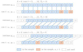
The staircase also exposes a detail that the population algebra handled quietly. At h=1, row 4 has s_4=0, so it sits in the comparison group, yet its outcome is y_5, which contains the intervention s_5. That is the term \theta_0s_{t+1} inside u_{t,1} in Equation 7. In population it does no harm, because s_5 is unrelated to s_4; in a sample of ten rows it is one more source of noise in the comparison.

In Stata the three regressions are a three-line loop over the hand table:

import delimited using hand_table.csv, clear asdouble   // variables t s v y
tsset t
forvalues h = 0/2 {
    regress F`h'.y s if t >= 2
}

6.2 The Slope as a Difference in Means

With a binary intervention, Equation 10 simplifies to arithmetic that can be done by hand. Suppose n_1 of the n rows have s_t=1 and the other n_0=n-n_1 have s_t=0, and write \bar y_1 and \bar y_0 for the mean of y_{t+h} in the two groups. Then \bar s=n_1/n, and the denominator of the slope is

\sum_t(s_t-\bar s)^2=n_1\Bigl(1-\frac{n_1}{n}\Bigr)^2+n_0\Bigl(\frac{n_1}{n}\Bigr)^2 =\frac{n_1n_0}{n}.

For the numerator, split the sum into the two groups:

\sum_t(s_t-\bar s)\,y_{t+h} =n_1\bar y_1-\frac{n_1}{n}\bigl(n_1\bar y_1+n_0\bar y_0\bigr) =\frac{n_1n_0}{n}\bigl(\bar y_1-\bar y_0\bigr).

Dividing the second display by the first,

\hat\beta_h=\bar y_1-\bar y_0 . \tag{14}

The slope is the mean outcome h periods after intervention rows minus the mean outcome h periods after the other rows, and the intercept is \bar y_0. Equation 12 is the special case n_1=1.

In the hand table, Equation 14 needs only group sums. At h=0 the rows are t=2,\dots,12 and the intervention rows are 5, 10, and 12. Their outcomes sum to y_5+y_{10}+y_{12}=3.792626953125, so \bar y_1=1.264208984375. The eight other outcomes sum to 5.17509765625, so \bar y_0=0.64688720703125, and \hat\beta_0=0.61732177734375. At h=1 the last row is 11, so row 12 and its intervention have left the sample. The intervention rows are 5 and 10, whose outcomes are y_6 and y_{11}: \bar y_1=-0.06982421875/2=-0.034912109375, \bar y_0=7.587548828125/8=0.948443603515625, and \hat\beta_1=-0.983355712890625. At h=2 the rows end at 10, the intervention rows are again 5 and 10 with outcomes y_7 and y_{12}: \bar y_1=4.565087890625/2=2.2825439453125, \bar y_0=1.62763671875/7=0.23251953125, and \hat\beta_2=2.0500244140625. Table 4 collects the results.

Table 4: Slopes computed from the rows of the twelve-period economy, rounded to six decimals from exact values. Without the control each slope is the difference in means of Equation 14; with y_{t-1} included it is no longer a difference in means.

h	T_h	Rows	Intervention rows	\bar y_1	\bar y_0	\hat\beta_h, no control	\hat\beta_h, with y_{t-1}	\theta_h
0	11	2–12	5, 10, 12	1.264209	0.646887	0.617322	0.575667	1
1	10	2–11	5, 10	−0.034912	0.948444	−0.983356	−1.050405	0.5
2	9	2–10	5, 10	2.282544	0.232520	2.050024	2.153022	0.25

Stata’s regress returns 0.61732179, -0.98335569, and 2.05002437. The differences in the eighth decimal come from floating-point storage¹², not from the arithmetic. Adding y_{t-1} changes the slopes to 0.575667, -1.050405, and 2.153022, on the same rows. Exercise 3 builds these rows by hand, and Exercise 4 reproduces them in Stata with assertions.

None of the six estimates is close to its target. The impact estimate is 0.62 against 1, the h=1 estimate has the wrong sign, and the h=2 estimate is eight times too large. Equation 11 explains why. With two or three intervention rows, the weighted sum of everything else is dominated by a few disturbances: the h=1 intervention rows have outcomes y_6 and y_{11}, and y_6 carries half of y_5, with its disturbance of -1.7, while y_{11} receives v_{11}=-0.9. The arithmetic of a local projection is the same in a sample of twelve periods as in a sample of two hundred. What changes is how many rows vote and how much of the noise their votes cancel.

7 Reading the Response Graph

The hand table produced three numbers. A response is usually read as a curve, and a curve raises two new problems. It needs one regression per horizon, organized so that every coefficient stays attached to the rows behind it. And it needs labels, because a curve by itself does not say what a unit of the intervention is, what the vertical axis measures, or what the comparison is.

7.1 From One Regression per Horizon to a Curve

Take one simulated sample from Equation 3 with \rho=0.9 and \theta_0=\sigma_s=\sigma_v=1: 300 periods drawn with seed 2, the intervention drawn before the disturbance, and the first 100 periods discarded, so T=200. The same 200 observations are shipped with the browser lab and the practicum, so every medium works with identical rows. A loop estimates the response for h=0,\dots,12 and stores each coefficient with its sample size:

import delimited using onedraw_rho09_seed2.csv, clear   // variables t s v y
tsset t
tempname P
postfile `P' h double beta_h T_h using results_onedraw, replace
forvalues h = 0/12 {
    quietly regress F`h'.y s L.y
    post `P' (`h') (_b[s]) (e(N))
}
postclose `P'
use results_onedraw, clear
assert T_h == 199 - h

Storing e(N) in the same post as _b[s] is what keeps each coefficient and its row count together. The assertion checks Equation 13 with T=200 and p=1; if a missing value had crept into the data, the loop would still run, and only the assertion would notice. Exercise 6 runs this loop and draws the graph, and Exercise 7 wraps it in a Monte Carlo experiment.

7.2 What a Response Graph Must Say

A response graph plots \hat\beta_h against h. Four pieces of information are needed to read it, and the curve supplies none of them.

1. The intervention and its units. A coefficient is a response per unit of s, so the reader must know what one unit is. Here it is one unit of the simulated intervention, which is also one standard deviation because \sigma_s=1.
2. The outcome’s units. The vertical axis is in units of y; in data it might be percent, percentage points, or points of trend GDP, and Lecture 2 shows how easily those are confused.
3. The horizon unit. The horizontal axis counts periods after the intervention, with h=0 the period of the intervention itself.
4. The counterfactual. The vertical axis measures the gap from the path without the intervention. A value of zero means “no different from that path,” not “the outcome is zero” and not “the outcome is back where it started.”

The intercept \mu_h is not on the graph and is not the counterfactual path. It absorbs means and says nothing about what would have happened without the intervention. A complete caption fills the four slots and leaves the intercept out; Figure 4 is captioned that way.

Figure 4: One sample against the truth. Response of y to a one-unit (one standard deviation) intervention s_t, estimated by local projections with y_{t-1} as the control in one simulated sample of T=200 periods with \rho=0.9 (seed 2). Horizons are periods after the intervention; the vertical axis is the gap from the path without the intervention, in units of y. The true response is \theta_h=0.9^h. The band holds the middle 90 percent of estimates across R=500 simulated samples (stored simulation result, seed 3). This sample’s estimates lie below \theta_h at every horizon.

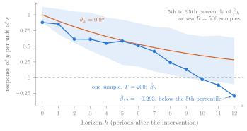
The sample gives \hat\beta_0=0.878940, \hat\beta_4=0.548477, \hat\beta_8=0.240595, and \hat\beta_{12}=-0.293297, against \theta_h=1, 0.6561, 0.4305, and 0.2824. Every one of the thirteen estimates is below its target, and from h=8 on the shortfall grows steadily, from 0.19 to 0.58. Read on its own, the curve says that the response turns negative after ten periods. The true response is positive at every horizon.

The 5–95 percent band¹³ shows how unusual this sample is. Across 500 simulated samples, 90 percent of the estimates at h=8 lie between 0.047 and 0.793, so a sample of 200 periods can deliver almost any value in that range. This sample sits just below the band’s lower edge at h=0, stays inside it from h=1 through h=10, and falls below it at h=11 and h=12. The seed was fixed before any estimate was computed, and the draw is kept because its failure is informative: the errors at neighbouring horizons are not independent. Adjacent regressions use almost the same rows, and Section 8 shows that their residuals share most of their terms. When one horizon’s estimate is too low, its neighbours tend to be too low as well.

The same 500 samples also show where the estimates are centred. With \rho=0.5, the mean estimate is within 0.014 of \theta_h at every horizon. With \rho=0.9 it falls systematically short: by 0.026 at h=4, 0.033 at h=8, and 0.049 at h=12. The Monte Carlo standard error¹⁴ of those means is about 0.01, so the gap at h=12 is almost five times its standard error. It is the small-sample bias already visible in Table 2, and Lecture 2 explains it.

The graph still lacks what a published response graph normally shows: a band computed from the sample itself. The band in Figure 4 used knowledge of the true economy that no researcher has. A band built from one sample has to start from the residual, and the residual has a structure of its own.

8 What the Residual Contains

The estimates in Figure 4 erred in the same direction at every horizon. The source of that pattern is visible in Equation 7 once the residuals of two rows are written side by side.

8.1 Shared Terms Between Rows

Start with h=1. Row t and the next row have residuals

u_{t,1}=\rho\,v_t+v_{t+1}+\theta_0s_{t+1}, \qquad u_{t+1,1}=\rho\,v_{t+1}+v_{t+2}+\theta_0s_{t+2}.

The disturbance v_{t+1} appears in both, with weight 1 in row t and weight \rho in row t+1. Every other term is distinct and independent. With \theta_0=\sigma_s=\sigma_v=1, the covariance of the two residuals is therefore \rho and each variance is \rho^2+1+1=2+\rho^2, so their correlation is \rho/(2+\rho^2). Rows two periods apart share nothing, and their residuals are uncorrelated.

The reason is timing, not misspecification. The outcome of row t is dated t+1 and the outcome of row t+1 is dated t+2, but row t’s residual reaches forward to t+1, into the period that row t+1’s residual also covers. A regression of outcomes h periods ahead on data sampled every period builds overlapping windows, and overlapping windows share disturbances.

The same counting works at any horizon. For 1\le k\le h, rows t and t+k share the disturbances v_{t+k},\dots,v_{t+h} and the interventions s_{t+k+1},\dots,s_{t+h}. A shared disturbance v_{t+j} enters row t with weight \rho^{h-j} and row t+k with weight \rho^{h-j+k}, so it contributes \rho^k\rho^{2(h-j)}\sigma_v^2 to the covariance. Summing these geometric terms over j=k,\dots,h, and doing the same for the shared interventions over j=k+1,\dots,h, gives

\operatorname{Cov}\bigl(u_{t,h},u_{t+k,h}\bigr)= \begin{cases} \rho^{k}\,\dfrac{\sigma_v^2\bigl(1-\rho^{2(h-k+1)}\bigr)+\theta_0^2\sigma_s^2\bigl(1-\rho^{2(h-k)}\bigr)}{1-\rho^2}, & 0\le k\le h,\\[2ex] 0, & k>h. \end{cases} \tag{15}

At k=0 the first line is the variance of u_{t,h}. Read the formula from the outside in. The factor \rho^k discounts for the distance between the rows; the fraction counts how much of the two windows overlaps, which shrinks as k approaches h; and beyond k=h the windows no longer meet. With \theta_0=\sigma_s=\sigma_v=1 and h=2, the variance is 2+2\rho^2+\rho^4 and the covariances at k=1 and k=2 are 2\rho+\rho^3 and \rho^2. Table 5 turns these into correlations and checks them against the residuals of a long simulated sample.

Table 5: Autocorrelations of the horizon-h residual. Formula values come from Equation 15 with \theta_0=\sigma_s=\sigma_v=1; simulated values are the sample autocorrelations of least-squares residuals in one sample of T=100{,}000 periods (seed 4).

Residual and lag	\rho=0.5, formula	\rho=0.5, simulated	\rho=0.9, formula	\rho=0.9, simulated
u_{t,1}, lag 1	0.2222	0.2213	0.3203	0.3216
u_{t,1}, lag 2	0	0.0019	0	0.0038
u_{t,2}, lag 1	0.4390	0.4375	0.5914	0.5911
u_{t,2}, lag 2	0.0976	0.0980	0.1894	0.1911
u_{t,2}, lag 3	0	0.0011	0	0.0011

The residual of a horizon-h regression is therefore correlated with its own values up to h rows away and uncorrelated beyond. In the language of time series it is at most a moving average of order h¹⁵. The correlation grows with the horizon, because longer windows overlap more, and with persistence, because shared terms are discounted less. At h=20, the longest horizon used with the quarterly data below, the toy economy’s residual is correlated with the residuals of the twenty rows on either side. Exercise 8 derives the \rho=0.5 entries of Table 5.

8.2 Shared Terms Across Horizons

The same row’s residuals at neighbouring horizons are linked even more tightly. Comparing Equation 7 at h and h+1,

u_{t,h+1}=\rho\,u_{t,h}+v_{t+h+1}+\theta_0s_{t+h+1}.

The horizon-(h+1) residual is \rho times the horizon-h residual plus one new period. With \rho=0.9, most of what went wrong at one horizon carries into the next. By Equation 11, the estimation errors are weighted sums of these residuals over nearly the same rows, so they inherit the link. That is why the curve in Figure 4 sat below the truth everywhere instead of scattering around it: a response graph is not thirteen independent estimates, and a pattern across neighbouring horizons can be a single error drawn thirteen times.

8.3 What This Does and Does Not Imply

Serially correlated residuals usually prompt a worry about standard errors, and the worry is not wrong. But Equation 11 shows that what enters the estimate is the residual multiplied by the intervention, not the residual alone. Consider the products s_tu_{t,h} and s_{t+k}u_{t+k,h} for k\ge1. The intervention s_t appears in neither residual and not in s_{t+k}, it is independent of all of them, and it has mean zero, so the expected product of the two terms is zero. The products are uncorrelated even though the residuals are not. Lecture 5 shows that inference on \beta_h depends on the autocorrelation of s_tu_{t,h}, which in this economy is zero because s_t is independent of everything else in both products and the control y_{t-1} keeps earlier interventions out of the residual, and it examines what changes when either fails (Montiel Olea and Plagborg-Møller, 2021).

This lecture records the structure and stops there. The toy economy has done its work. Beyond this point no known response is available to check an estimate against, and the regression meets the data the lecture began with.

9 First Contact with Data

The opening asked what military news did to output. We now run the local projection Equation 9 on the quarterly data behind that question, with \mathbf w_t=y_{t-1} exactly as in the simulations: least squares of y_{t+h} on a constant, s_t, and y_{t-1}, one regression for each h=0,\dots,20.

9.1 The Data and Their Units

The data are Ramey and Zubairy’s quarterly U.S. series for 1889Q1–2015Q4, 508 quarters, from the rzdat sheet of RZDAT.xlsx in their February 2018 replication package (Ramey and Zubairy, 2018). The workbook’s readme sheet is dated November 21, 2016, and the package’s jordagk.do describes the file as updated April 7, 2016. The course does not redistribute the file: Practicum 01 downloads it from the authors’ archive and verifies its checksum, and the browser lab displays only estimates computed from it.

The outcome is real GDP divided by trend GDP, y_t=\texttt{rgdp}_t/\texttt{rgdp\_pott6}_t. Both series are in billions of chained 2009 dollars¹⁶ at an annual rate, so y_t has no units and averages 0.987 over the sample. A change of 0.01 in y_t is a change in GDP of one percent of trend GDP.

The intervention variable is the military news,

s_t=\frac{\texttt{news}_t}{\texttt{rgdp\_pott6}_{t-1}\times\texttt{pgdp}_{t-1}},

the change in the expected present value of military spending announced in quarter t, in billions of nominal dollars, divided by the previous quarter’s nominal trend GDP at an annual rate. Military news¹⁷ is recorded by the quarter in which it arrived, which is why it is dated t and the control y_{t-1} one quarter earlier. The series is nonmissing from 1890Q1 to 2015Q4, 504 quarters, and nonzero in only 108 of them. Its mean is 0.007222 and its standard deviation 0.059728. The two largest values are 0.691893 in 1941Q4 and 0.600073 in 1950Q3. A unit of s_t is news worth a full year of trend GDP, so coefficients are best read per 0.01: news worth one percent of trend GDP.

Counting rows needs one adjustment to Equation 13. Row t needs s_t, which starts in 1890Q1, and y_{t-1}, which exists there because GDP starts four quarters earlier. The lag therefore costs no row, and the horizon-h regression has T_h=504-h rows, from 1890Q1 to h quarters before 2015Q4. The formula counts a lag as a lost row only when the lagged variable begins where the sample does.

9.2 A Hump

The estimates rise from \hat\beta_0=0.080313 at impact to \hat\beta_4=0.259141 and \hat\beta_8=0.361906, peak at \hat\beta_{10}=0.404210, and fall back to 0.0796 by h=20. Figure 5 plots them.

Figure 5: Military news and GDP, first contact. Response of real GDP, in percent of trend GDP, to military-spending news worth one percent of the previous quarter’s nominal trend GDP, from regressions of y_{t+h} on a constant, the news, and y_{t-1} over 1890Q1–2015Q4 (T_h=504-h). Numerically this is \hat\beta_h per unit of the scaled news variable. Horizons are quarters after the news arrives. Read causally, the vertical axis is the gap from the path without the news, a reading this section lists as not yet argued. The response peaks at 0.404 at h=10. With Ramey and Zubairy’s controls (four lags each of news, GDP, and government spending, both relative to trend), the h=10 coefficient is 0.294. No bands are shown.

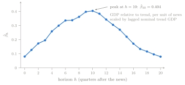
In words: news worth one percent of trend GDP is followed ten quarters later by GDP about 0.40 percent of trend GDP above what the regression otherwise predicts from the previous quarter’s output. The shape is a hump, which Section 3 showed an AR(1) cannot produce, and the local projection found it without being told what shape to expect.

Changing the controls changes the numbers. With Ramey and Zubairy’s own set, so that \mathbf w_t in Equation 9 holds four lags each of the news, of y, and of government spending relative to trend (p=4), the sample becomes T_h=500-h and the coefficients are 0.0510 at h=0, 0.2938 at h=10, and 0.0671 at h=20. These equal, to the digits shown, the linear GDP response in Ramey and Zubairy’s replication code, which Lecture 4 reproduces. The peak falls by about a quarter. Which of the two specifications deserves a causal reading, if either, is not a question the regression can answer.

9.3 Where the Variation Comes From

Equation 10 says that each quarter supplies the share (s_t-\bar s)^2/\sum_\tau(s_\tau-\bar s)^2 of the variation behind the slope. Table 6 lists the six largest shares in the h=8 sample of 496 quarters.

Table 6: The six quarters with the largest shares of \sum_t(s_t-\bar s)^2 in the h=8 estimation sample, 1890Q1–2013Q4 (T_8=496). Shares use s_t-\bar s as in Equation 10; with y_{t-1} in the regression, the exact weights use s_t purged of y_{t-1}. Rounded to four decimals.

Quarter	News, fraction of trend GDP	Share of variation	Cumulative share
1941Q4	0.6919	0.2612	0.2612
1950Q3	0.6001	0.1958	0.4570
1942Q3	0.4328	0.1009	0.5579
1950Q4	0.4022	0.0869	0.6448
1917Q2	0.3729	0.0745	0.7193
1941Q2	0.3401	0.0617	0.7811

The quarter of Pearl Harbor and the first full quarter of the Korean War supply 45.7 percent of the variation in s_t between them; four quarters supply 64.5 percent and six supply 78.1 percent. Of 496 rows, a handful carry the estimate. The data are closer to the one-episode case of Equation 12 than their length suggests.

A direct test confirms it. At h=8 the estimate is 0.3619 on the full sample. Dropping the single row for 1950Q3 raises it to 0.4340, so one quarter out of 496 moves the coefficient by 0.072. Dropping 1941Q4 instead gives 0.3443, and dropping both gives 0.4451. Using only rows from 1947Q1 on, 268 of them, gives 0.0587. Removing Korea’s news quarter raises the estimate: measured against the regression’s average, what followed the Korean news was smaller than what followed the other large episodes. And most of what the full-sample coefficient reports comes from before 1947. Exercise 9 reproduces the response, the shares, and the drop-one estimate from the data.

9.4 What Has Not Yet Been Argued

Figure 5 is a response graph, and its caption names the intervention, the units, and the counterfactual. It is not yet evidence about what military news does to output. At least five claims stand between the estimate and that conclusion, and each belongs to a later lecture.

1. Units and transformation. The outcome is a level relative to a trend fitted with data through 2015, and the coefficient is per unit of scaled news. Whether the level, the change, or the accumulated response answers the policymaker’s question, and what units each carries, is Lecture 2.
2. Controls. One lag of y was a choice. Ramey and Zubairy’s controls lower the peak by a quarter, and which controls belong depends on what drives the news, which is Lecture 3.
3. Identification. The argument that equated the coefficient with \theta_h required the news to be an observed shock in the sense of A2 and A3: unpredictable from the past and unrelated to the taxes, monetary policy, price controls, and war that arrived with it. Lecture 3 argues about that, and Lecture 4 uses the news to estimate the effect of spending itself.
4. Uncertainty. No standard error or band has been computed. Overlapping windows make the residuals serially correlated, and Lectures 5 and 6 build intervals that respect what Section 8 found.
5. Episode dependence. Two quarters carry 46 percent of the variation, and dropping one moves the h=8 estimate by 0.07. Lecture 13 turns this into a systematic sensitivity analysis.

A sixth claim is hidden in A1. The regression treats news worth 69 percent of trend GDP as having 69 times the effect of news worth one percent, in slack and in booming economies alike; Lectures 9 and 10 ask what a linear coefficient means when that fails.

10 Handoff

The policymaker of June 1950 wanted to know what the buildup would do to output. The lecture cannot answer that question yet, but it can now say precisely what a local projection offers in reply. Each coefficient compares what followed quarters with more news against what followed quarters with less, holding the previous quarter’s output fixed. In an economy where the news is an observed shock, that comparison equals the gap between the realized path and the path without the news. The coefficients are estimated one horizon at a time from rows that shrink as the horizon grows. Their variation comes from every quarter with news, weighted by how unusual the news was, and in these data a few war quarters dominate.

The opening’s evidence can now be set beside the regression. The realized rise in output from 1950Q2 to 1953Q1 was 0.0787 of trend GDP. Scaling the h=10 coefficient by Korea’s news gives 0.600073\times0.404210=0.2426, three times larger. Neither number is the effect of Korea’s news. The first is a change along one realized path, which Equation 2 splits into a response and everything else. The second applies an average over many episodes, led by 1941Q4, to one of them, with controls and identification unargued. Exercise 10 asks you to take the comparison apart.

We can now produce a defined estimand, a derivation showing when a regression recovers it, the rows of that regression listed by hand, a loop that estimates the curve, and a response graph whose caption says what it measures. We cannot yet defend a choice of the outcome’s form. Every regression in this lecture used the level y_{t+h}. The opening’s 7.87 points was a change, y_{t+h}-y_{t-1}, and Section 1 insisted that a change since the date before is not a causal response. Yet y_{t-1} also sits on the right-hand side of the regression behind every response graph we drew. If we regress y_{t+h}-y_{t-1} instead of y_{t+h}, is the answer different, or the same answer in different clothes? Lecture 2 begins there.

Exercises

Exercises marked [core] prepare material used later in the course.

Exercise 1: Two paths, one difference

Problem. [core, pencil] The twelve-period economy of the notes follows y_t=0.5\,y_{t-1}+s_t+v_t with y_0=0, and its interventions fall at t=1,5,10,12. Around the second intervention the realized path is y_4=0.0625, y_5=-0.66875, y_6=-0.134375, y_7=2.0328125, and y_8=-0.28359375, and the disturbances are v_5=-1.7, v_6=0.2, v_7=2.1, and v_8=-1.3.

1. Build the counterfactual path y^{c}_t for t=5,\dots,8 by switching off the intervention at t=5 and nothing else. Tabulate y_t, y^{c}_t, the gap y_t-y^{c}_t, and the change since the date before, y_t-y_4.

2. Split each change y_t-y_4 into the causal response and the change the economy would have made without the intervention. At which dates does reading the change as the effect get the sign wrong, and by what factor does it overstate the effect at t=7?

3. Without repeating the recursion, give the four gaps that would result if every v_t were replaced by zero, and explain why.

TipHint

Only one input differs between the two recursions: s_5 equals 1 on the realized path and 0 on the counterfactual one. Start both paths from y_4, which an intervention dated t=5 cannot have moved, and feed the same v_t into both. For (c), subtract one recursion from the other before substituting any number.

NoteDetailed solution

The two paths obey the same rule and receive the same disturbances:

y_t=0.5\,y_{t-1}+s_t+v_t, \qquad y^{c}_t=0.5\,y^{c}_{t-1}+s^{c}_t+v_t,

with s^{c}_5=0 and s^{c}_t=s_t at every other date. Before t=5 the rule never uses s_5, so the paths coincide up to that date and y^{c}_4=y_4=0.0625. The plan is to run the second recursion forward from there and compare.

(a) Four applications of the rule give the counterfactual path:

\begin{aligned} y^{c}_5&=0.5(0.0625)+0-1.7=-1.66875,\\ y^{c}_6&=0.5(-1.66875)+0+0.2=-0.634375,\\ y^{c}_7&=0.5(-0.634375)+0+2.1=1.7828125,\\ y^{c}_8&=0.5(1.7828125)+0-1.3=-0.40859375. \end{aligned}

Every input has a short decimal expansion, so the table is exact; nothing is rounded.

t	y_t	y^{c}_t	Gap y_t-y^{c}_t	Change y_t-y_4	y^{c}_t-y_4
5	−0.66875	−1.66875	1	−0.73125	−1.73125
6	−0.134375	−0.634375	0.5	−0.196875	−0.696875
7	2.0328125	1.7828125	0.25	1.9703125	1.7203125
8	−0.28359375	−0.40859375	0.125	−0.34609375	−0.47109375

The gap is measured in units of y for a one-unit intervention. Its halving can be read off the two rules. Subtracting the counterfactual rule from the realized one,

y_t-y^{c}_t=0.5\,\bigl(y_{t-1}-y^{c}_{t-1}\bigr)+\bigl(s_t-s^{c}_t\bigr),

and the disturbance has cancelled. At t=5 the gap is 0.5\times0+1=1; after that s_t-s^{c}_t=0, so each period keeps half of the previous gap.

(b) Add and subtract y^{c}_t:

y_t-y_4=\underbrace{\bigl(y_t-y^{c}_t\bigr)}_{\text{causal response}} +\underbrace{\bigl(y^{c}_t-y_4\bigr)}_{\text{change without the intervention}}.

The last three columns of the table carry out the split. At t=5, -0.73125=1+(-1.73125); at t=7, 1.9703125=0.25+1.7203125. The second bracket contains no intervention at all. Iterating the counterfactual rule from t=4 gives y^{c}_7=0.5^3y_4+0.5^2v_5+0.5\,v_6+v_7=0.0078125-0.425+0.1+2.1, so the counterfactual change 1.7203125 is the fading of y_4 plus three disturbances, and v_7=2.1 alone is larger than all of it.

Reading the change as the effect gets the sign wrong at t=5 (-0.73125 against 1), at t=6 (-0.196875 against 0.5), and at t=8 (-0.34609375 against 0.125). At t=7 it reports 1.9703125 against 0.25, which is 7.88125 times the effect. The intervention did the same thing at every date; the disturbances did not.

(c) The gap recursion in (a) contains no v_t. Replacing every disturbance by zero moves both paths but leaves their difference alone, so the gaps are still 1, 0.5, 0.25, and 0.125. They are the formula \theta_h=\theta_0\rho^h from the notes’ section on the smallest model, with \theta_0=1 and \rho=0.5, read at h=0,\dots,3. This is the check on the whole calculation: a gap that changed when the disturbances changed would signal an arithmetic slip.

Two mistakes are common. The first is the one the lecture opens with: reporting y_5-y_4=-0.73125 as the effect of the intervention. The second is to build the counterfactual by setting s_t=0 at every date, as if “no intervention” meant no interventions at all. The intervention at t=1 then disappears as well, its fading contribution 0.5^{t-1} joins each gap, and the gaps become 1.0625, 0.53125, 0.265625, and 0.1328125. The causal response to one intervention removes that intervention and nothing else.

Exercise 2: Iterate forward

Problem. [core, pencil] Let y_t=\rho\,y_{t-1}+\theta_0s_t+v_t, where the interventions s_t and the disturbances v_t each have mean zero, are independent over time, and are independent of each other, and |\rho|<1 (Assumptions A1–A4 of the notes).

1. Substitute the rule into itself to write y_{t+1} and then y_{t+2} in terms of y_{t-1} and the interventions and disturbances dated t onward. State the general formula for y_{t+h} and prove it by induction.

2. Change s_t by one unit while holding y_{t-1}, every disturbance, and every other intervention fixed. Derive the causal response \theta_h.

3. For the population regression of y_{t+h} on (1,s_t,y_{t-1}), read off \mu_h, \beta_h, \gamma_h, and the residual u_{t,h} from your formula. Show that \mathbb E[u_{t,h}]=\mathbb E[s_tu_{t,h}]=\mathbb E[y_{t-1}u_{t,h}]=0, and name the assumption each step uses.

4. With \theta_0=1 and \rho=0.9, compute \theta_4 and \theta_7, and find the first horizon at which the response is below half of its impact value.

TipHint

Do two substitutions by hand before writing any sum, and watch what the second substitution does to every term the first one produced. That operation is the induction step. For (c), write down the date of every term in u_{t,h} before taking a single expectation.

NoteDetailed solution

The object we want is y_{t+h} written as “the pre-intervention outcome, plus everything that arrives from t onward.” The rule gives each outcome in terms of the previous one, so we replace the previous outcome repeatedly until only y_{t-1} is left.

(a) At h=0 the rule itself is already in that form. For h=1, write the rule one period later and substitute for y_t:

\begin{aligned} y_{t+1}&=\rho\,y_t+\theta_0s_{t+1}+v_{t+1}\\ &=\rho\bigl(\rho\,y_{t-1}+\theta_0s_t+v_t\bigr)+\theta_0s_{t+1}+v_{t+1}\\ &=\rho^2y_{t-1}+\rho\,\theta_0s_t+\rho\,v_t+\theta_0s_{t+1}+v_{t+1}. \end{aligned}

For h=2, write y_{t+2}=\rho\,y_{t+1}+\theta_0s_{t+2}+v_{t+2} and substitute the last line:

y_{t+2}=\rho^3y_{t-1}+\rho^2\theta_0s_t+\rho^2v_t+\rho\,\theta_0s_{t+1} +\rho\,v_{t+1}+\theta_0s_{t+2}+v_{t+2}.

The second substitution multiplied every existing term by \rho and appended the new period’s intervention and disturbance with coefficient one. Repeating that operation suggests

y_{t+h}=\rho^{h+1}y_{t-1}+\sum_{j=0}^{h}\rho^{h-j}\bigl(\theta_0s_{t+j}+v_{t+j}\bigr).

Induction. At h=0 the formula reads \rho\,y_{t-1}+\theta_0s_t+v_t, which is the rule. Suppose it holds at h. Then

\begin{aligned} y_{t+h+1}&=\rho\,y_{t+h}+\theta_0s_{t+h+1}+v_{t+h+1}\\ &=\rho^{h+2}y_{t-1}+\sum_{j=0}^{h}\rho^{h+1-j}\bigl(\theta_0s_{t+j}+v_{t+j}\bigr) +\rho^{0}\bigl(\theta_0s_{t+h+1}+v_{t+h+1}\bigr), \end{aligned}

and the last term is the j=h+1 term of the sum at horizon h+1. The formula therefore holds at h+1, and so at every horizon.

(b) The intervention s_t appears only in the j=0 term of the sum, with coefficient \rho^h\theta_0. Raising s_t by one unit with everything else fixed raises y_{t+h} by that coefficient, so

\theta_h=\theta_0\rho^h,

in units of y per unit of s. The rule is linear and its coefficients do not depend on the date (A1), so the response is the same for every t and for any starting value of s_t.

(c) Match the formula with y_{t+h}=\mu_h+\beta_hs_t+\gamma_hy_{t-1}+u_{t,h}. The proposal is \mu_h=0, \beta_h=\theta_0\rho^h, \gamma_h=\rho^{h+1}, and everything left over is the residual:

u_{t,h}=\sum_{j=0}^{h}\rho^{h-j}v_{t+j}+\theta_0\sum_{j=1}^{h}\rho^{h-j}s_{t+j}.

Its terms are dated as follows: the disturbances v_t,\dots,v_{t+h} and the interventions s_{t+1},\dots,s_{t+h}. The second sum starts at j=1 because s_t has moved into the \beta_h term. A proposal is the population projection if its residual satisfies the three orthogonality conditions, because only one set of coefficients does when s_t and y_{t-1} both vary and neither is an exact linear function of the other. Here \sigma_s^2>0 (A2), and y_{t-1}, built from terms dated t-1 or earlier, varies and is uncorrelated with s_t (A2, A3).

1. Mean zero. Every v_{t+j} and every s_{t+j} has mean zero (A2, A3), so \mathbb E[u_{t,h}]=0.
2. Orthogonal to s_t. The product s_tu_{t,h} is a sum of terms s_tv_{t+j} with j\ge0 and s_ts_{t+j} with j\ge1. The first kind has expectation \mathbb E[s_t]\,\mathbb E[v_{t+j}]=0 because the two sequences are independent (A3). The second kind has expectation \mathbb E[s_t]\,\mathbb E[s_{t+j}]=0 because interventions are independent over time with mean zero (A2).
3. Orthogonal to y_{t-1}. Iterating the rule backward, y_{t-1}=\sum_{i\ge0}\rho^i(\theta_0s_{t-1-i}+v_{t-1-i}), a sum that settles down because |\rho|<1 (A4). Every term of y_{t-1} is dated t-1 or earlier, every term of u_{t,h} is dated t or later, and by A2 and A3 the two groups are independent. Each term of u_{t,h} has mean zero, so \mathbb E[y_{t-1}u_{t,h}]=0.

All three conditions hold, so the projection coefficients are \mu_h=0, \beta_h=\theta_h=\theta_0\rho^h, and \gamma_h=\rho^{h+1}. As a special-case check, at h=0 the residual is u_{t,0}=v_t, \beta_0=\theta_0, and \gamma_0=\rho: the projection is the rule itself.

Two of the three steps used the assumptions about how interventions and disturbances arise, and none used anything about least squares. That is where the causal content of \beta_h=\theta_h sits.

(d) With \theta_0=1 and \rho=0.9,

\theta_4=0.9^4=0.6561, \qquad \theta_7=0.9^7=0.4782969.

The response falls below half of its impact value when 0.9^h<0.5, that is, when h>\ln0.5/\ln0.9=6.58 (rounded to two decimals). The first such horizon is h=7; one period earlier, \theta_6=0.531441 is still above one half. The control’s coefficient over the same horizons is \gamma_h=0.9^{h+1}, for example \gamma_4=0.59049, but it measures the fading of the pre-intervention outcome, not a response to anything.

Three slips recur. Starting the intervention sum in u_{t,h} at j=0 puts s_t into the residual, which makes \mathbb E[s_tu_{t,h}]=\theta_0\rho^h\sigma_s^2 and suggests a bias that does not exist. Writing \gamma_h=\rho^h forgets that y_{t-1} has had h+1 periods to fade. And attributing \mathbb E[y_{t-1}u_{t,h}]=0 to A2 alone overlooks that y_{t-1} contains past disturbances, so A3 is needed as well.

Exercise 3: Rows by hand

Problem. [core, pencil] In the twelve-period economy the interventions are s_t=1 at t=1,5,10,12 and s_t=0 otherwise, and the realized outcomes are

t	y_t	t	y_t	t	y_t
1	1.9	5	−0.66875	9	0.658203125
2	1.45	6	−0.134375	10	1.9291015625
3	1.325	7	2.0328125	11	0.06455078125
4	0.0625	8	−0.28359375	12	2.532275390625

For h=0,1,2, consider the regression of y_{t+h} on a constant and s_t, using only rows with t\ge2 so that y_{t-1} would exist in every row.

1. List the rows of each regression and give T_h. Check your count against T_h=T-h-p.

2. Identify the intervention rows and compute the mean of y_{t+h} over the intervention rows, \bar y_1, and over the other rows, \bar y_0.

3. Compute \hat\beta_h and compare it with \theta_h=0.5^h.

4. Row 4 of the h=1 regression sits in the comparison group. What is its outcome, and why is that outcome not a clean comparison?

TipHint

Draw the staircase before computing anything. For each h, write t in one column and t+h in the next, then strike out every row whose outcome date passes 12. Only after that sort the surviving rows by s_t.

NoteDetailed solution

A regression row is dated by its intervention: row t pairs s_t with the outcome y_{t+h}. Row t needs the lag y_{t-1}, which exists only for t\ge2 because y_0 is not part of the data, and the lead y_{t+h}, which exists only for t\le12-h. The plan is to fix those rows first, then use the fact from the notes that with a 0–1 regressor the least-squares slope is the difference in means, \hat\beta_h=\bar y_1-\bar y_0.

(a) The rows are t=2,\dots,12 at h=0, t=2,\dots,11 at h=1, and t=2,\dots,10 at h=2, so T_0=11, T_1=10, and T_2=9. With T=12 and one lag, p=1, the formula gives T_h=12-h-1: 11, 10, and 9. Each horizon costs the last row, and the lag costs row 1 at every horizon.

(b) At h=0 the intervention rows are 5, 10, and 12. At h=1 row 12 has left the sample, because its outcome y_{13} does not exist, and the intervention rows are 5 and 10; they remain 5 and 10 at h=2. Each row contributes its outcome h periods later:

• h=0. Intervention outcomes y_5,y_{10},y_{12} sum to 3.792626953125, so \bar y_1=1.264208984375. The eight other outcomes y_2,y_3,y_4,y_6,y_7,y_8,y_9,y_{11} sum to 5.17509765625, so \bar y_0=0.64688720703125.
• h=1. Intervention outcomes y_6 and y_{11} sum to -0.06982421875, so \bar y_1=-0.034912109375. The eight other rows t=2,3,4,6,7,8,9,11 have outcomes y_3,y_4,y_5,y_7,y_8,y_9,y_{10},y_{12}, which sum to 7.587548828125, so \bar y_0=0.948443603515625.
• h=2. Intervention outcomes y_7 and y_{12} sum to 4.565087890625, so \bar y_1=2.2825439453125. The seven other rows t=2,3,4,6,7,8,9 have outcomes y_4,y_5,y_6,y_8,y_9,y_{10},y_{11}, which sum to 1.62763671875, so \bar y_0=0.23251953125.

(c) Subtracting,

\hat\beta_0=0.61732177734375,\qquad \hat\beta_1=-0.983355712890625,\qquad \hat\beta_2=2.0500244140625.

h	T_h	Rows	Intervention rows	\bar y_1	\bar y_0	\hat\beta_h	\theta_h
0	11	2–12	5, 10, 12	1.264209	0.646887	0.617322	1
1	10	2–11	5, 10	−0.034912	0.948444	−0.983356	0.5
2	9	2–10	5, 10	2.282544	0.232520	2.050024	0.25

The table rounds to six decimals; the display above it is exact. The slopes are in units of y per unit of s. None is close to its target: the impact estimate is 0.62 against 1, the h=1 estimate has the wrong sign, and the h=2 estimate is eight times too large. Two or three intervention rows cannot average away disturbances such as v_5=-1.7 and v_7=2.1.

Check. The covariance form of the slope must agree. At h=0, \bar s=3/11, so \sum_t(s_t-\bar s)^2=n_1n_0/n=3\times8/11=24/11, and \sum_t(s_t-\bar s)\,y_t=1.346883877841 (rounded to twelve decimals). Their ratio is 0.617321777\ldots, the same slope. The intercept of each regression equals \bar y_0, which is a second check.

(d) Row 4 has s_4=0, so it belongs to the comparison group, but its outcome at h=1 is y_5=0.5\,y_4+s_5+v_5=-0.66875, which contains the intervention at t=5. In the notation of the notes this is the term \theta_0s_{t+1} inside the residual u_{t,1}. Rows 9 and 11 have the same feature: their outcomes y_{10} and y_{12} contain the interventions at t=10 and t=12, while neither intervention row has an intervention one period later. Through that term alone, the comparison mean \bar y_0 carries three units of intervention spread over eight rows, which adds 3/8=0.375 to \bar y_0 and lowers \hat\beta_1 by the same amount. In population this does no harm, because s_{t+1} is independent of s_t and averages out across many rows. In ten rows it does not average out.

The most common slip is to compute \bar y_1 minus the mean of all rows instead of the mean of the other rows. That gives (n_0/n)(\bar y_1-\bar y_0)=(8/11)\times0.61732177734375=0.448961\ldots at h=0. Another is to leave row 12 in the h=1 regression with a blank outcome treated as zero, which adds a fictitious intervention row.

Exercise 4: The same rows in Stata

Problem. [core, computational] Reproduce the regressions of Exercise 3 in Stata, then add the lagged outcome as a control on the same rows. Write a do-file that

1. enters the twelve rows of the hand table (the values of s_t and v_t are s_t=1 at t=1,5,10,12 and v_t=0.9,\,0.5,\,0.6,\,-0.6,\,-1.7,\,0.2,\,2.1,\,-1.3,\,0.8,\,0.6,\,-0.9,\,1.5), rebuilds y_t from y_t=0.5\,y_{t-1}+s_t+v_t with y_0=0, and declares the data with tsset t;

2. loops over h=0,1,2 with forvalues, computes \bar y_1 and \bar y_0 with summarize, and runs regress F`h'.y s if t >= 2 with and without L.y, storing h, T_h, and both slopes;

3. asserts that T_h=11-h in both regressions, that the slope without the control equals \bar y_1-\bar y_0 to within 10^{-6}, that both regressions use exactly the same rows, and that the slopes without the control equal those of Exercise 3.

Report the three slopes with the control and explain why they are no longer differences in means.

TipHint

Check e(N) before you look at any coefficient. Stata’s F. operator returns a missing value past the last period and regress drops such rows without comment, so the row count is the first thing that can go wrong. Ask, too, which rows the regression with L.y loses that the one without it keeps.

NoteDetailed solution

The do-file below types the rows rather than drawing them, so it depends on neither a data file nor a random-number stream. It stores v_t and y_t as double, for a reason given at the end. The assertions sit where the claims of Exercise 3 are made: the row count right after each regression, the difference in means before the slope is stored, and the comparison of samples before the control’s slope is posted.

* ex04_hand_rows.do  Lecture 01, Exercise 4: the hand-table rows in Stata
* Run from the lab project's top folder with StataNow/SE 19.5.
version 19
clear all
set more off
capture log close
log using output/ex04_hand_rows.txt, text replace

* The twelve rows of the hand table, typed from the notes. Storing v and y
* as double keeps Stata's arithmetic equal to the exact decimals.
input byte t byte s double v
 1 1  0.9
 2 0  0.5
 3 0  0.6
 4 0 -0.6
 5 1 -1.7
 6 0  0.2
 7 0  2.1
 8 0 -1.3
 9 0  0.8
10 1  0.6
11 0 -0.9
12 1  1.5
end
tsset t
generate double y = s + v in 1                  // y_0 = 0
replace y = 0.5*L.y + s + v in 2/12
assert abs(y[5]  - (-0.66875))     < 1e-12   // check the typed rows
assert abs(y[12] - 2.532275390625) < 1e-12

tempname P
postfile `P' h T_h n1 n0 double(ybar1 ybar0 b_noctrl b_ctrl) ///
    using output/ex04_results, replace
forvalues h = 0/2 {
    * group means of the outcome h periods ahead, rows t >= 2
    quietly summarize F`h'.y if t >= 2 & s == 1
    local ybar1 = r(mean)
    local n1 = r(N)
    quietly summarize F`h'.y if t >= 2 & s == 0
    local ybar0 = r(mean)
    local n0 = r(N)

    * the regression without the control
    quietly regress F`h'.y s if t >= 2
    assert e(N) == 11 - `h'                     // T_h = T - h - p
    assert `n1' + `n0' == e(N)
    assert abs(_b[s] - (`ybar1' - `ybar0')) < 1e-6
    assert abs(_b[_cons] - `ybar0') < 1e-6
    local b_noctrl = _b[s]
    tempvar rows
    generate byte `rows' = e(sample)

    * the regression with y_(t-1), which must use the same rows
    quietly regress F`h'.y s L.y if t >= 2
    assert e(N) == 11 - `h'
    quietly count if e(sample) != `rows'
    assert r(N) == 0
    post `P' (`h') (e(N)) (`n1') (`n0') (`ybar1') (`ybar0') ///
        (`b_noctrl') (_b[s])
    drop `rows'
}
postclose `P'

use output/ex04_results, clear
format ybar1 ybar0 b_noctrl b_ctrl %12.8f
list, clean noobs

* exact slopes from the notes; with-control slopes to six decimals
assert n1 == cond(h == 0, 3, 2)
assert abs(b_noctrl - 0.61732177734375)     < 1e-9 if h == 0
assert abs(b_noctrl - (-0.983355712890625)) < 1e-9 if h == 1
assert abs(b_noctrl - 2.0500244140625)      < 1e-9 if h == 2
assert abs(b_ctrl - 0.575667)    < 5e-7 if h == 0
assert abs(b_ctrl - (-1.050405)) < 5e-7 if h == 1
assert abs(b_ctrl - 2.153022)    < 5e-7 if h == 2
display "Exercise 4: all assertions passed"
log close

Run in StataNow/SE 19.5, every assertion passes. The listing in the log is:

    h   T_h   n1   n0         ybar1        ybar0      b_noctrl        b_ctrl
    0    11    3    8    1.26420898   0.64688721    0.61732178    0.57566739
    1    10    2    8   -0.03491211   0.94844360   -0.98335571   -1.05040519
    2     9    2    7    2.28254395   0.23251953    2.05002441    2.15302246

Without the control, each slope is the difference in means of Exercise 3, printed to eight decimals: 0.61732178 is 0.61732177734375 rounded. The row counts confirm T_h=T-h-p, and the group sizes confirm that row 12’s intervention leaves at h=1.

With y_{t-1} included, the slopes are 0.575667, -1.050405, and 2.153022 (rounded to six decimals), on exactly the same rows. They are no longer differences in means. By the Frisch–Waugh–Lovell result that the notes preview in a footnote, the slope now uses s_t after removing its linear relation to y_{t-1} in these rows. In population that relation is zero, because the intervention is independent of the previous outcome (A2 and A3). In nine to eleven rows it is not exactly zero, so the control moves the three estimates by 0.04, 0.07, and 0.10 in absolute value (rounded to two decimals). The control’s own coefficients tell the same story: exact least squares on these rows gives \hat\gamma_0=-0.061, \hat\gamma_1=-0.115, and \hat\gamma_2=0.233 (rounded to three decimals), against \rho^{h+1}=0.5, 0.25, and 0.125. The population coefficient the two regressions target is the same, \beta_h=\theta_h; neither estimate comes near it in twelve periods.

Why the tolerance. With double storage, Stata’s slopes agree with exact decimal arithmetic to about 10^{-15}, so even the 10^{-9} assertions pass. Stored as float, which is what generate and input use by default, v_t becomes a binary approximation such as 0.89999998; delete double from the input and generate lines to see it. The slopes then print as 0.61732179, -0.98335569, and 2.05002437, the values the notes quote, because the shipped hand_table.csv was generated from float draws. They still satisfy every 10^{-6} assertion, while the 10^{-12} checks on the typed rows and the 10^{-9} checks on the slopes fail, as they should. A test written as assert _b[s] == ybar1 - ybar0 would be testing storage, not the regression.

What the first assertion catches. Leaving out if t >= 2 changes one regression but not the other. At h=0 the regression without the control then uses all twelve rows, including row 1 with its intervention, and returns 0.7762695 (rounded to seven decimals). The regression with L.y still uses eleven rows, because y_0 is missing. The two slopes would differ in their rows as well as in their control, and the first assertion, e(N) == 11 - h, stops the do-file before anyone compares them.

Exercise 5: One episode

Problem. [core, pencil] Replace the intervention column of the hand table by an indicator that equals 1 at t=5 and 0 at every other date, and keep the rows t\ge2 and the outcomes listed in Exercise 3.

1. Show that when exactly one of n rows, row \tau, has the indicator equal to 1, the least-squares slope of y_{t+h} on a constant and the indicator is y_{\tau+h}-\bar y_{\text{others}}, where \bar y_{\text{others}} is the mean outcome over the other n-1 rows.

2. Compute the slope at h=0,1,2 and compare each with \theta_h=0.5^h.

3. Use the forward equation y_{\tau+h}=\theta_h+\rho^{h+1}y_{\tau-1}+u_{\tau,h} to split the h=0 slope into \theta_0 and everything else. Which term dominates?

4. Return to the original intervention column (s_t=1 at t=1,5,10,12). As h grows, the regression of y_{t+h} on s_t over rows t\ge2 becomes a single-episode regression without any change to the data. At which horizon does that first happen, and what is the slope there?

TipHint

With a single intervention row, the “mean of the intervention rows” is one outcome. Start from the difference-in-means result of Exercise 3 with n_1=1, or compute \bar s, \sum_t(s_t-\bar s)^2, and the weight on each row directly.

NoteDetailed solution

(a) The slope on a 0–1 regressor is the difference in means, so with one intervention row \bar y_1=y_{\tau+h} and \bar y_0=\bar y_{\text{others}}, and the result follows at once. The weights make the same point more concretely. With one intervention among n rows, \bar s=1/n and

\sum_t(s_t-\bar s)^2=\Bigl(1-\frac1n\Bigr)^2+(n-1)\frac{1}{n^2} =\frac{(n-1)^2+(n-1)}{n^2}=\frac{n-1}{n}.

The slope is \sum_t\omega_ty_{t+h} with \omega_t=(s_t-\bar s)/\sum_\tau(s_\tau-\bar s)^2. Row \tau gets \omega_\tau=(1-1/n)\big/\bigl((n-1)/n\bigr)=1, and every other row gets -(1/n)\big/\bigl((n-1)/n\bigr)=-1/(n-1). Hence

\hat\beta_h=y_{\tau+h}-\frac{1}{n-1}\sum_{t\neq\tau}y_{t+h} =y_{\tau+h}-\bar y_{\text{others}}.

The episode’s outcome gets full weight, and the other rows share a weight of -1 equally.

(b) At h=0 the rows are t=2,\dots,12, so n=11. The episode’s outcome is y_5=-0.66875, and the ten other outcomes sum to 9.636474609375, a mean of 0.9636474609375. At h=1 (n=10) the episode’s outcome is y_6=-0.134375, and the nine others, y_3,y_4,y_5,y_7,\dots,y_{12}, sum to 7.652099609375, a mean of 0.850233289\ldots. At h=2 (n=9) the episode’s outcome is y_7=2.0328125, and the eight others, y_4,y_5,y_6,y_8,\dots,y_{12}, sum to 4.159912109375, a mean of 0.519989013671875. So

\hat\beta_0=-1.6323974609375,\qquad \hat\beta_1=-0.984608\ldots,\qquad \hat\beta_2=1.512823486328125,

or -1.632397, -0.984608, and 1.512823 rounded to six decimals, against \theta_h=1, 0.5, and 0.25. Two estimates have the wrong sign and the third is six times too large.

(c) At \tau=5 and h=0 the forward equation is the rule itself: y_5=\theta_0+\rho\,y_4+u_{5,0} with u_{5,0}=v_5. Substituting \theta_0=1, \rho\,y_4=0.5\times0.0625=0.03125, and v_5=-1.7,

\hat\beta_0=\underbrace{1}_{\theta_0} +\underbrace{\bigl(0.03125-1.7-0.9636474609375\bigr)}_{\text{everything else}} =1+(-2.6323974609375)=-1.6323974609375.

Everything else is more than twice the response, and the episode’s own disturbance, -1.7, is by itself larger than \theta_0. The same split works at h=1: y_6=\theta_1+\rho^2y_4+u_{5,1} with u_{5,1}=\rho\,v_5+v_6+\theta_0s_6=-0.85+0.2+0=-0.65, so \hat\beta_1=0.5+(0.015625-0.65-0.850233\ldots)=0.5+(-1.484608\ldots). The data contain one number at each horizon. Nothing in them says how much of it is \theta_h and how much is the bracket.

(d) At h=3 the rows are t=2,\dots,9. Row 10 and row 12 have no outcome three periods later, and row 1 is excluded, so row 5 is the only intervention row left. The original regression is then exactly the single-episode regression, and part (a) applies to it unchanged:

\hat\beta_3=y_8-\frac{y_5+y_6+y_7+y_9+y_{10}+y_{11}+y_{12}}{7} =-0.28359375-\frac{6.413818359375}{7}=-1.199853515625,

against \theta_3=0.125. This is also a check on (a): the slope from the difference-in-means formula of Exercise 3 and the slope from the one-episode formula must coincide here, and they do. Row 5 stays the only intervention row through h=7, so the regressions at h=4,\dots,7, on 7, 6, 5, and 4 rows, are single-episode regressions as well. At h=8 the rows are t=2,3,4, none of them has an intervention, s_t does not vary, and no slope can be computed; Stata’s regress reports s as omitted because of collinearity.

The Korean episode in the notes has the same structure, with taxes, the Treasury–Federal Reserve Accord, and price controls inside the bracket.

It is easy to subtract the mean of all n rows, including the episode itself. That shrinks the answer by the factor (n-1)/n: at h=0 it gives (10/11)\times(-1.6323974609375)=-1.483998 (rounded to six decimals). The error is small here, but it hides the logic of the formula, which compares the episode with everything else.

Exercise 6: A response in a loop

Problem. [core, computational] The Practicum 01 lab project ships data/raw/onedraw_rho09_seed2.csv, one simulated sample of T=200 periods from y_t=0.9\,y_{t-1}+s_t+v_t with \sigma_s=\sigma_v=1 (seed 2; variables t, s, v, y). Lab 3 of the Shock-to-Response Explorer displays the same observations.

1. Write a do-file that loops over h=0,\dots,12, regresses y_{t+h} on a constant, s_t, and y_{t-1}, and stores h, \hat\beta_h, and T_h with postfile.

2. Assert that T_h=199-h, that \hat\beta_0=0.878940 and \hat\beta_{12}=-0.293297 to within 10^{-6}, and state how many of the thirteen estimates lie below \theta_h=0.9^h.

3. Draw the response graph with \theta_h overlaid and write a caption that names the intervention and its units, the units of the outcome, the horizon unit, and the counterfactual.

4. In two or three sentences, say what the graph shows about this sample and what it cannot show.

TipHint

Put e(N) in the same post command as _b[s], so each coefficient travels with the number of rows behind it. For the caption, fill four slots before writing a sentence: what one unit of the intervention is, what the vertical axis measures, what the horizontal axis counts, and what a value of zero is being compared with.

NoteDetailed solution

One regression per horizon produces one point on the curve, so the loop has thirteen regressions and a results file with thirteen rows. The design decision that matters most is to store each coefficient together with its sample size and to test the sample size before trusting the coefficient.

* ex06_loop.do  Lecture 01, Exercise 6: a response in a loop
* Run from the lab project's top folder with StataNow/SE 19.5.
version 19
clear all
set more off
capture log close
log using output/ex06_loop.txt, text replace

import delimited using data/raw/onedraw_rho09_seed2.csv, clear   // t s v y
tsset t
assert _N == 200

tempname P
postfile `P' h double beta_h T_h using output/results_onedraw, replace
forvalues h = 0/12 {
    quietly regress F`h'.y s L.y
    post `P' (`h') (_b[s]) (e(N))          // coefficient with its rows
}
postclose `P'

use output/results_onedraw, clear
generate double theta_h = 0.9^h
assert T_h == 199 - h                        // T - h - p, T = 200, p = 1
assert abs(beta_h[1]  - 0.878940)    < 1e-6  // h = 0
assert abs(beta_h[13] - (-0.293297)) < 1e-6  // h = 12
quietly count if beta_h < theta_h
assert r(N) == 13                            // below the truth at every h
format beta_h theta_h %9.6f
list h T_h beta_h theta_h, clean noobs

twoway (line theta_h h, lcolor(gs8) lpattern(dash))                  ///
       (connected beta_h h, lcolor(navy) mcolor(navy) msize(small)), ///
       yline(0, lcolor(gs13))                                        ///
       xlabel(0(2)12) ylabel(-0.4(0.2)1, format(%3.1f) angle(0))     ///
       xtitle("Horizon h (periods after the intervention)")          ///
       ytitle("Gap from the no-intervention path (units of y)")      ///
       legend(order(2 "Estimate, this sample"                        ///
                    1 "True response 0.9{sup:h}") rows(1) position(6)) ///
       graphregion(color(white)) plotregion(color(white))
graph export output/ex06_response.pdf, replace
display "Exercise 6: all assertions passed"
log close

The assertions pass, and the log lists:

     h   T_h      beta_h    theta_h
     0   199    0.878940   1.000000
     1   198    0.853260   0.900000
     2   197    0.612737   0.810000
     3   196    0.611046   0.729000
     4   195    0.548477   0.656100
     5   194    0.583099   0.590490
     6   193    0.509120   0.531441
     7   192    0.417788   0.478297
     8   191    0.240595   0.430467
     9   190    0.130293   0.387420
    10   189   -0.028821   0.348678
    11   188   -0.117200   0.313811
    12   187   -0.293297   0.282430

An independent least-squares calculation in Python on the same CSV reproduces all thirteen coefficients to the six decimals shown. All thirteen estimates lie below \theta_h. In the exported graph the connected estimate starts near 0.88 and runs below the dashed truth by between 0.01 and 0.20 through h=8 (rounded to two decimals). After that the gap widens at every step, and the estimate is negative from h=10 on while 0.9^h stays positive.

A caption that does its job. “Response of y to a one-unit intervention s_t (one unit is one standard deviation, since \sigma_s=1), estimated by local projections of y_{t+h} on a constant, s_t, and y_{t-1} in one simulated sample of T=200 periods with \rho=0.9 (seed 2). Horizons are periods after the intervention; h=0 is the period in which it occurs. The vertical axis is the gap between the path with the intervention and the path without it, in units of y. The dashed line is the true response \theta_h=0.9^h. No sampling uncertainty is shown.” Each of the four slots is filled: the intervention and its unit, the outcome’s units, the horizon unit, and the counterfactual that zero refers to.

What the graph shows and what it does not. In this sample the estimated response is below the truth at every horizon. The shortfall grows from 0.19 at h=8 to 0.58 at h=12 (rounded to two decimals), and a reader shown only this curve would say the effect turns negative at h=10. The graph cannot say whether the sample is typical. Neighbouring estimates share almost all their rows and most of their residual terms, so a curve that errs in one direction at every horizon may be one error seen thirteen times. Only the distribution across many samples, which Exercise 7 builds, or a band computed from the sample itself, which Lectures 5 and 6 build, can separate the two.

The mistake to expect here is in the caption rather than the code. Writing “response of y” on the vertical axis without saying that zero means “no different from the path without the intervention” invites the reading that zero means “y is back where it started”. The graph measures gaps between paths, not changes along one.

Exercise 7: Many draws

Problem. [computational] Wrap the loop of Exercise 6 in a Monte Carlo experiment. Each sample comes from y_t=\rho\,y_{t-1}+s_t+v_t with y_0=0 and s_t and v_t independent standard normal draws: 300 periods, all 300 values of s drawn before any v (generate s = rnormal(), then generate v = rnormal()), the first 100 periods discarded, so T=200. Set the seed to 3 once for each \rho\in\{0.5,0.9\}, outside the replication loop, and expose the number of replications as global R with a default of 200. In each sample, estimate \hat\beta_h for h=0,\dots,12 with y_{t-1} (199-h rows) and without it, on every row that has the lead (200-h rows).

1. For each \rho and h, report the mean, standard deviation, and 5th and 95th percentiles of \hat\beta_h with the control, and the mean and standard deviation without it. With R=200, assert that at \rho=0.9 and h=8 the mean and standard deviation with the control are 0.370337 and 0.211226 to within 10^{-6}.

2. Using the Monte Carlo standard error, the standard deviation divided by \sqrt R, decide at which horizons the mean differs from \theta_h=\rho^h by more than simulation noise.

3. Compare the spread with and without the control at each \rho. Explain the pattern with the variance of the term \rho^{h+1}y_{t-1} that the regression without the control leaves in its residual.

4. Where does the sample of Exercise 6 lie relative to the 5–95 percent band at h=8 and at h=12?

TipHint

Post every estimate with its replication number, \rho, h, and e(N), and compute summaries after the loop from the stored estimates rather than inside it. For (c), work out \rho^{2(h+1)}\operatorname{Var}(y) at h=0 and h=4 for both values of \rho before you look at the simulated standard deviations.

NoteDetailed solution

A Monte Carlo experiment answers a question one sample cannot: how an estimator behaves when the true response is known. The design fixes everything except the draws, so differences across replications are sampling variation and differences between the mean and \theta_h are properties of the estimator. Seeding once per design makes the R=200 run the first 200 replications of the same stream as the notes’ R=500 table.

* ex07_many_draws.do  Lecture 01, Exercise 7: many draws
* Run from the lab project's top folder with StataNow/SE 19.5.
version 19
clear all
set more off
capture log close
log using output/ex07_many_draws.txt, text replace

if "$R" == "" global R 200          // replications (D2 student default)
timer clear 1
timer on 1

tempname P
postfile `P' rep double rho h double(b_ctrl b_noctrl) n_ctrl n_noctrl ///
    using output/mc_draws, replace
foreach rho in 0.5 0.9 {
    set seed 3                      // once per design, before the loop
    quietly forvalues r = 1/$R {
        clear
        set obs 300
        generate t = _n
        tsset t
        generate s = rnormal()                  // s first, then v
        generate v = rnormal()
        generate y = s + v in 1
        replace y = `rho'*L.y + s + v in 2/300
        drop if t <= 100                        // burn-in of 100 periods
        replace t = _n
        tsset t
        forvalues h = 0/12 {
            regress F`h'.y s L.y
            local b_c = _b[s]
            local n_c = e(N)
            regress F`h'.y s
            post `P' (`r') (`rho') (`h') (`b_c') (_b[s]) (`n_c') (e(N))
        }
    }
}
postclose `P'
timer off 1
quietly timer list 1
display "Monte Carlo runtime: " %6.1f r(t1) " seconds for R = $R"

use output/mc_draws, clear
assert n_ctrl == 199 - h & n_noctrl == 200 - h
generate double theta_h = rho^h
collapse (mean) theta_h mean_ctrl=b_ctrl mean_noctrl=b_noctrl ///
         (sd) sd_ctrl=b_ctrl sd_noctrl=b_noctrl               ///
         (p5) p5=b_ctrl (p95) p95=b_ctrl, by(rho h)
generate double bias = mean_ctrl - theta_h
generate double mcse = sd_ctrl/sqrt($R)
format theta_h mean_* sd_* p5 p95 bias mcse %9.6f
list rho h theta_h mean_ctrl bias mcse sd_ctrl p5 p95 ///
    mean_noctrl sd_noctrl, clean noobs
save output/mc_R${R}_summary, replace

* checks
assert sd_noctrl > sd_ctrl if rho == 0.9   // the control buys precision
assert abs(bias) < 3*mcse if rho == 0.5 & h <= 4
if $R == 200 {
    assert abs(mean_ctrl - 0.370337) < 1e-6 if rho == 0.9 & h == 8
    assert abs(sd_ctrl   - 0.211226) < 1e-6 if rho == 0.9 & h == 8
}
display "Exercise 7: all assertions passed"
log close

Two runs took 27.3 and 27.8 seconds in StataNow/SE 19.5, and every assertion passed in both. The no-control regressions use 200-h rows, one more than the controlled ones, because they do not need y_0; this matches the design behind the notes’ table. Selected rows of the summary, rounded to four decimals:

\rho	h	\theta_h	Mean	MCSE	SD	5th pct.	95th pct.	Mean, no control	SD, no control
0.5	0	1.0000	1.0028	0.0051	0.0717	0.8800	1.1171	0.9994	0.0970
0.5	4	0.0625	0.0507	0.0085	0.1208	−0.1459	0.2439	0.0548	0.1217
0.5	8	0.0039	−0.0169	0.0083	0.1173	−0.2065	0.1901	−0.0172	0.1178
0.5	12	0.0002	−0.0105	0.0085	0.1197	−0.2034	0.1764	−0.0120	0.1206
0.9	0	1.0000	1.0031	0.0051	0.0720	0.8783	1.1135	0.9690	0.2209
0.9	4	0.6561	0.6279	0.0134	0.1899	0.3424	0.9418	0.6219	0.2651
0.9	8	0.4305	0.3703	0.0149	0.2112	0.0608	0.6944	0.3705	0.2568
0.9	12	0.2824	0.2303	0.0155	0.2185	−0.1138	0.6167	0.2320	0.2449

(a) The log prints the asserted cell at full precision: at \rho=0.9 and h=8 the mean is 0.370337 and the standard deviation 0.211226. Every estimate is in units of y per unit of s, and one unit of s is one standard deviation.

(b) The Monte Carlo standard error measures how far a simulated mean could plausibly lie from the mean that unlimited replications would give. Divide each gap between the mean estimate and \theta_h by its MCSE, and read a ratio beyond about two as more than simulation noise. At \rho=0.9 every mean from h=1 to h=12 is below \theta_h, and the ratio passes two at h=2 and at every horizon from h=4 on. The gap at h=2 is -0.0233, 2.2 standard errors; at h=4 it is -0.0282, 2.1; from h=5 on, every gap is between 2.9 and 4.0 standard errors, the largest being -0.0601 at h=8. Only h=0, 1, and 3 stay inside two. That is more than simulation noise: the estimator with T=200 falls systematically short at this persistence, by more at long horizons than at short ones, which is the small-sample bias Lecture 2 takes up.

At \rho=0.5 the ratio also passes two at four horizons: h=2, 5, 7, and 8, at 2.2, 2.8, 2.0, and 2.5 standard errors, with the largest gap -0.0241 at h=5. These gaps stay within 0.025 of \theta_h, about a fifth of the estimator’s standard deviation, and they do not grow with h. Thirteen correlated comparisons easily produce a few ratios of that size, and the notes’ R=500 run puts every gap at \rho=0.5 within 0.014. A small shortfall at \rho=0.5 cannot be ruled out, but at its largest it is less than half the one at \rho=0.9. One caution applies to both readings: the thirteen means come from the same samples, so their errors are correlated and the ratios are not thirteen independent tests.

(c) With \rho=0.9 the control cuts the spread at impact by a factor of three, from 0.2209 to 0.0720. Those are close to the large-sample values in the notes, \sqrt{9.53/200}=0.218 and 1/\sqrt{199}=0.071. The ratio of the two standard deviations falls with the horizon, to 1.40 at h=4, 1.22 at h=8, and 1.12 at h=12 (rounded to two decimals). The means with and without the control are close at h=4, 8, and 12; the control changes the spread much more than the centre.

The omitted term explains both patterns. Without the control, the residual carries \rho^{h+1}y_{t-1}, whose variance is \rho^{2(h+1)}\operatorname{Var}(y) with \operatorname{Var}(y)=(\theta_0^2\sigma_s^2+\sigma_v^2)/(1-\rho^2). At \rho=0.9, \operatorname{Var}(y)=10.53, and the added variance is still 3.67 at h=4. At \rho=0.5, \operatorname{Var}(y)=2.67 and the added variance at h=4 is 0.0026. So at \rho=0.5 the control matters most at impact, 0.0717 against 0.0970, a little at h=1 and h=2, where the ratios are 1.13 and 1.07, and hardly at all after that. From h=4 on the two standard deviations are within one percent of each other, and at h=5 and h=6 the one without the control is even slightly smaller, which is simulation noise.

(d) In Exercise 6, \hat\beta_8=0.240595 lies inside the band from 0.0608 to 0.6944, below the centre but not unusually so. At h=12, \hat\beta_{12}=-0.293297 lies below the 5th percentile, -0.1138. The same sample is ordinary at one horizon and unusual four horizons later. That fits what the notes say about the residual: neighbouring estimates share rows and residual terms, so a sample that starts low tends to stay low and can drift out of the band.

Seeding inside the loop. Putting set seed 3 inside the replication loop resets the generator in every replication. Each replication then draws the same sample, so the experiment is a single seed-3 sample estimated two hundred times. A standard deviation of exactly zero at every horizon is the symptom.

Exercise 8: What the residual contains

Problem. [core, pencil] In the AR(1) economy with \theta_0=\sigma_s=\sigma_v=1, the horizon-h residual of the regression on (1,s_t,y_{t-1}) is u_{t,h}=\sum_{j=0}^{h}\rho^{h-j}v_{t+j}+\sum_{j=1}^{h}\rho^{h-j}s_{t+j}.

1. Write u_{t,1} and u_{t+1,1} term by term, list the terms they share, and derive \operatorname{Corr}(u_{t,1},u_{t+1,1}) as a function of \rho.

2. Write u_{t,2} and u_{t+k,2} for k=1,2,3. Count the shared terms and compute \operatorname{Corr}(u_{t,2},u_{t+k,2}) at \rho=0.5 for each k.

3. Explain in one or two sentences why the correlation is zero beyond lag h.

4. Show that \mathbb E[s_tu_{t,2}\,s_{t+1}u_{t+1,2}]=0, even though u_{t,2} and u_{t+1,2} are correlated.

TipHint

Write the two residuals one above the other, aligned by date, with each term’s weight. A covariance collects only the terms that appear in both rows, and each shared term contributes the product of its two weights.

NoteDetailed solution

Every term of a residual is either a disturbance v or an intervention s, each with variance one, and all of them are mutually independent (A2 and A3). So the variance of a residual is the sum of its squared weights, and the covariance of two residuals is the sum, over the terms they share, of the products of the two weights. Nothing else enters.

(a) At h=1,

u_{t,1}=\rho\,v_t+v_{t+1}+s_{t+1}, \qquad u_{t+1,1}=\rho\,v_{t+1}+v_{t+2}+s_{t+2}.

The rows share one term, v_{t+1}, with weight 1 in row t and weight \rho in row t+1. Each variance is \rho^2+1+1=2+\rho^2, and the covariance is 1\times\rho=\rho. Hence

\operatorname{Corr}(u_{t,1},u_{t+1,1})=\frac{\rho}{2+\rho^2},

which at \rho=0.5 is 0.5/2.25=2/9=0.2222 (rounded to four decimals).

(b) At h=2 the terms and weights are:

Residual	v_t	v_{t+1}	v_{t+2}	v_{t+3}	v_{t+4}	s_{t+1}	s_{t+2}	s_{t+3}	s_{t+4}
u_{t,2}	\rho^2	\rho	1			\rho	1
u_{t+1,2}		\rho^2	\rho	1			\rho	1
u_{t+2,2}			\rho^2	\rho	1			\rho	1

and u_{t+3,2} contains v_{t+3},v_{t+4},v_{t+5} and s_{t+4},s_{t+5}. The variance of each residual is

\operatorname{Var}(u_{t,2})=\rho^4+\rho^2+1+\rho^2+1=2+2\rho^2+\rho^4 .

• Lag 1. Rows t and t+1 share three terms: v_{t+1} (weights \rho and \rho^2), v_{t+2} (1 and \rho), and s_{t+2} (1 and \rho). The covariance is \rho^3+\rho+\rho=2\rho+\rho^3.
• Lag 2. Rows t and t+2 share one term, v_{t+2} (1 and \rho^2), so the covariance is \rho^2.
• Lag 3. Row t+3 begins at date t+3, after row t’s last term. Nothing is shared, and the covariance is zero.

At \rho=0.5 the variance is 2+0.5+0.0625=2.5625=41/16, and

\begin{aligned} \operatorname{Corr}(u_{t,2},u_{t+1,2})&=\frac{1.125}{2.5625}=\frac{18}{41}=0.4390,\\ \operatorname{Corr}(u_{t,2},u_{t+2,2})&=\frac{0.25}{2.5625}=\frac{4}{41}=0.0976,\\ \operatorname{Corr}(u_{t,2},u_{t+3,2})&=0, \end{aligned}

with the decimals rounded to four places. These are the \rho=0.5 entries of the notes’ table of residual autocorrelations, where the long simulated sample gives 0.2213, 0.4375, 0.0980, and 0.0011. The same counting at \rho=0.9 gives 0.3203, 0.5914, and 0.1894, so the correlations grow with persistence.

(c) Row t’s residual contains terms dated t through t+h, and row t+k’s residual contains terms dated t+k through t+k+h. For k>h the two windows do not overlap, and independent terms with no overlap have zero covariance. The residual is therefore at most a moving average of order h.

(d) Look for s_t in the product s_t\,u_{t,2}\,s_{t+1}\,u_{t+1,2}. It appears once, as the first factor. It is not in u_{t,2}, whose interventions start at s_{t+1}; it is not s_{t+1}; and it is not in u_{t+1,2}. By A2 and A3, s_t is independent of the other three factors, so

\mathbb E\bigl[s_tu_{t,2}\,s_{t+1}u_{t+1,2}\bigr] =\mathbb E[s_t]\;\mathbb E\bigl[u_{t,2}\,s_{t+1}u_{t+1,2}\bigr]=0 .

Because each product also has mean zero, the covariance of the two products is zero while the residuals themselves have correlation 0.4390. The estimation error of \hat\beta_h is a weighted sum of residuals with weights built from the interventions, so it is these products, not the bare residuals, whose dependence matters for its variance. Lecture 5 builds standard errors on that fact.

A frequent error is to leave the interventions s_{t+1},\dots,s_{t+h} out of the residual. At h=2 and lag 1 that drops one shared term and two variance terms, and gives (\rho^3+\rho)/(\rho^4+\rho^2+1)=0.625/1.3125=0.4762 at \rho=0.5 instead of 0.4390. Another is to conclude from correlated residuals that \hat\beta_h is biased; part (d) and the orthogonality conditions of Exercise 2 show why it is not.

Exercise 9: First contact with military news

Problem. [data, computational] Ramey and Zubairy’s quarterly U.S. data are in the workbook RZDAT.xlsx, sheet rzdat, from their February 2018 replication package. The course does not redistribute the file; the Practicum 01 lab project ships data/raw/get_rz.do, which downloads it from the authors’ archive, checks its SHA-256, and prints manual download steps if the download fails. The variables you need are quarter (fractional years), rgdp (real GDP) and rgdp_pott6 (trend GDP, the series the authors call potential GDP and estimate as a sixth-degree polynomial trend in real GDP), both in billions of chained 2009 dollars at an annual rate, pgdp (the GDP deflator), and news (military news, billions of nominal dollars).

1. Run get_rz.do, import the sheet, keep quarters from 1889Q1 on, and declare quarterly dates.

2. Construct y_t=\texttt{rgdp}_t/\texttt{rgdp\_pott6}_t and s_t=\texttt{news}_t/(\texttt{rgdp\_pott6}_{t-1}\times\texttt{pgdp}_{t-1}). Assert that s_t has 504 nonmissing values.

3. Estimate the local projection of y_{t+h} on a constant, s_t, and y_{t-1} for h=0,\dots,20, storing \hat\beta_h and T_h. Assert T_h=504-h and explain why the formula T_h=T-h-p, applied with T=504 quarters of news and p=1, seems to predict one row fewer. Report \hat\beta_8, \hat\beta_{10}, and the peak horizon.

4. On the h=8 estimation sample, compute each quarter’s share of \sum_t(s_t-\bar s)^2 and list the six largest.

5. Re-estimate the h=8 regression without 1950Q3. Does removing Korea’s news quarter raise or lower the estimate?

6. Draw the response graph and write its caption. Then write a paragraph of five sentences headed “What has not yet been argued”: one sentence each on units, controls, identification, uncertainty, and dependence on a few episodes.

TipHint

Date the news by the quarter in which it arrived, and the control one quarter earlier. Before running any loop, list 1950Q2 and 1950Q3 and check by hand that the 1950Q3 value of s_t divides that quarter’s news by 1950Q2’s nominal trend GDP.

NoteDetailed solution

The do-file repeats the notes’ first contact with data, starting from the raw workbook. It adds a check wherever a quarterly data set can go wrong: the date sequence, the timing of the scaling, the row count, and one coefficient that an independent source can confirm.

* ex09_first_contact.do  Lecture 01, Exercise 9: first contact with data
* Run from the lab project's top folder with StataNow/SE 19.5.
version 19
clear all
set more off
capture log close
log using output/ex09_first_contact.txt, text replace

* 1. Data: fetch the workbook or verify the copy already there (D5, D35)
do data/raw/get_rz.do "data/raw"
import excel using data/raw/RZDAT.xlsx, sheet("rzdat") firstrow clear
drop if quarter < 1889
generate qdate = yq(1889, 1) + _n - 1
format qdate %tq
tsset qdate, quarterly
assert _N == 508
assert abs(quarter - (1889 + (_n - 1)/4)) < 1e-6   // consecutive quarters

* 2. Outcome, intervention, and (for the check in step 6) spending:
*    y = real GDP / trend GDP, newsy = news / lagged nominal trend GDP,
*    g = real government spending / trend GDP
generate double y     = rgdp/rgdp_pott6
generate double newsy = news/(L.rgdp_pott6*L.pgdp)
generate double g     = (ngov/pgdp)/rgdp_pott6
quietly count if newsy < .
assert r(N) == 504
quietly count if newsy != 0 & newsy < .
display "quarters with nonzero news: " r(N)
summarize y newsy

* 3. One regression per horizon, h = 0,...,20
tempname P
postfile `P' h double beta_h T_h using output/first_contact, replace
forvalues h = 0/20 {
    quietly regress F`h'.y newsy L.y
    post `P' (`h') (_b[newsy]) (e(N))
}
postclose `P'

* 4. Where the variation comes from: shares in the h = 8 sample
quietly regress F8.y newsy L.y
generate byte in8 = e(sample)
quietly summarize newsy if in8
generate double dev2 = (newsy - r(mean))^2 if in8
quietly summarize dev2
generate double share = dev2/r(sum)
gsort -share
generate double cumshare = sum(share)
format newsy share cumshare %9.6f
list qdate newsy share cumshare in 1/6, clean noobs
assert qdate[1] == tq(1941q4) & abs(share[1] - 0.261211) < 1e-6
assert qdate[2] == tq(1950q3) & abs(share[2] - 0.195838) < 1e-6
sort qdate

* 5. Drop one episode at h = 8
quietly regress F8.y newsy L.y if qdate != tq(1950q3)
display "h = 8 without 1950Q3: " %9.6f _b[newsy] "  (T_8 = " e(N) ")"
assert e(N) == 495 & abs(_b[newsy] - 0.433969) < 1e-6

* 6. Check against a source record: Ramey and Zubairy's controls at h = 10
*    equal irf_gdp_linear in the REP04 benchmark (their jordagk.do)
quietly regress F10.y newsy L(1/4).newsy L(1/4).y L(1/4).g
display "h = 10 with RZ controls: " %10.8f _b[newsy] "  (N = " e(N) ")"
assert e(N) == 490 & abs(_b[newsy] - 0.29376385) < 1e-6

* 7. The response, its checks, and the graph
use output/first_contact, clear
assert T_h == 504 - h
assert abs(beta_h[9]  - 0.361906) < 1e-6        // h = 8
assert abs(beta_h[11] - 0.404210) < 1e-6        // h = 10
quietly summarize beta_h
assert beta_h[11] == r(max)                     // the peak is at h = 10
format beta_h %9.6f
list h T_h beta_h, clean noobs

twoway connected beta_h h, lcolor(navy) mcolor(navy) msize(small)      ///
       yline(0, lcolor(gs13)) xlabel(0(4)20)                          ///
       ylabel(0(0.1)0.5, format(%3.1f) angle(0))                      ///
       xtitle("Quarters after the news arrives")                      ///
       ytitle("Percent of trend GDP, per news worth 1 percent")       ///
       graphregion(color(white)) plotregion(color(white))
graph export output/ex09_first_contact.pdf, replace
display "Exercise 9: all assertions passed"
log close

In the verification run the workbook was already in data/raw, and get_rz.do reported “Ramey-Zubairy data present in data/raw and verified (SHA-256).” Every later assertion passed.

(a)–(b) The sheet holds 564 rows; dropping those before 1889 leaves 508 consecutive quarters, 1889Q1–2015Q4, and the date assertion confirms that no quarter is missing or repeated. The log’s summary gives y_t a mean of 0.9868665 over 508 quarters and s_t a mean of 0.0072219 and standard deviation 0.0597282 over 504 quarters, 108 of them nonzero. The four missing values of s_t are the 1889 quarters, where news is missing. A unit of s_t is news worth a full year of nominal trend GDP, so the natural reading unit is 0.01, news worth one percent of trend GDP.

(c) The assertion T_h=504-h passes. The formula T_h=T-h-p with T=504 and p=1 would give 503-h, but it counts a lag as a lost row only when the lagged variable begins where the sample does. Here the first row with news is 1890Q1, and y_{t-1} exists there because GDP starts four quarters earlier. The lag costs nothing, and each horizon still costs one row at the end. The estimates rise from \hat\beta_0=0.080313 to \hat\beta_4=0.259141 and \hat\beta_8=0.361906, peak at \hat\beta_{10}=0.404210, and fall to \hat\beta_{20}=0.079552. News worth one percent of trend GDP moves s_t by 0.01 and the prediction for y_{t+h} by 0.01\hat\beta_h; since y is a ratio to trend GDP, that is \hat\beta_h percent of trend GDP. Ten quarters after such news, GDP is about 0.40 percent of trend GDP above what the regression otherwise predicts from the previous quarter’s output.

(d) The six largest shares of \sum_t(s_t-\bar s)^2 in the h=8 sample (496 quarters, 1890Q1–2013Q4) are, as the log lists them:

     qdate      newsy      share   cumshare
    1941q4   0.691893   0.261211   0.261211
    1950q3   0.600073   0.195838   0.457049
    1942q3   0.432791   0.100897   0.557946
    1950q4   0.402163   0.086893   0.644839
    1917q2   0.372915   0.074496   0.719335
    1941q2   0.340130   0.061734   0.781069

Two quarters supply 45.7 percent of the variation and six supply 78.1 percent. The shares use s_t-\bar s, as in the notes’ slope formula; with y_{t-1} in the regression the exact weights use s_t purged of y_{t-1}, which is close but not identical.

(e) Without 1950Q3 the h=8 estimate is 0.433969 on 495 rows, against 0.361906 on the full sample. Removing Korea’s news quarter raises the estimate by 0.072. Measured against the regression’s average relation, what followed the Korean news eight quarters later was smaller than what followed the other large episodes, so that quarter was pulling the slope down.

Check against a source record. With Ramey and Zubairy’s own controls (four lags each of the news, y, and government spending relative to trend), the h=10 coefficient is 0.29376385 on 490 rows. That equals, at 10^{-6}, the linear GDP response irf_gdp_linear at h=10 in the course’s REP04 benchmark. The benchmark comes from an unmodified run of the authors’ jordagk.do, lines 253–386 and 398–417 of the frozen package. The data construction therefore matches the authors’ to the digits shown, and the difference from 0.404 comes from the controls, not from the data.

(f) The exported graph is a hump: 0.08 at impact, a peak of 0.40 at ten quarters, and 0.08 again at twenty. A caption that states what the reader needs:

Response of real GDP, in percent of trend GDP, to military-spending news worth one percent of the previous quarter’s nominal trend GDP. Local projections of y_{t+h} on a constant, the news, and y_{t-1}, 1890Q1–2015Q4, with T_h=504-h rows at horizon h. Horizons are quarters after the news arrives. Read causally, the vertical axis is the gap between GDP and the path it would have followed without the news, a reading not yet argued. No bands are shown.

A paragraph that lists, without defending, what the graph has not earned:

What has not yet been argued. The coefficients are responses of a level relative to a fitted trend per unit of scaled news, and whether that level, its change, or its accumulation answers the policymaker’s question is not yet settled. One lag of GDP is a choice, and Ramey and Zubairy’s controls lower the ten-quarter coefficient from 0.404 to 0.294. Reading the curve as the effect of the news requires the news to be unpredictable and unrelated to the taxes, monetary policy, price controls, and wars that arrived with it, which nothing here has shown. No standard error or band has been computed, and the overlapping horizons make the residuals serially correlated. Two quarters, 1941Q4 and 1950Q3, supply 45.7 percent of the variation in the news, and dropping 1950Q3 alone moves the eight-quarter estimate from 0.362 to 0.434.

Each sentence points to a later lecture: units to Lecture 2, controls and identification to Lectures 3 and 4, uncertainty to Lectures 5 and 6, and episode dependence to Lecture 13.

Two mistakes are predictable. The first is a timing slip in the scaling: dividing the news by the same quarter’s nominal trend GDP, or lagging the news itself instead of its denominator. Either changes the variable the notes define, the second also dates every episode a quarter late, and the hand check on 1950Q3 in the hint catches both. The second mistake is to assert T_h=503-h from the formula and then “fix” the data until it passes, which throws away a quarter of real data. The formula counts rows that are missing; it does not decide which rows should be.

Exercise 10: Korea is not the average

Problem. [extra, pencil] In the Ramey–Zubairy data, GDP relative to trend was y=0.972500 in 1950Q2, and the news in 1950Q3 was s=0.600073 of lagged nominal trend GDP. Later values of y were 1.000572 in 1950Q3, 1.033931 in 1951Q3, and 1.051212 in 1953Q1. The first-contact local projection of Exercise 9 gives \hat\beta_0=0.080313, \hat\beta_4=0.259141, and \hat\beta_{10}=0.404210.

1. For h=0,4,10, compute the realized change y_{1950Q3+h}-y_{1950Q2} and the scaled coefficient 0.600073\,\hat\beta_h, both in units of trend GDP.

2. Which of the two numbers, if either, measures a gap between two paths?

3. Give three distinct reasons why the two numbers differ, and say what follows if both are taken at face value.

TipHint

Write each number as a difference between two outcomes, and label each outcome with its date and with the path it lies on, realized or counterfactual. For (c), look for reasons on both sides: in what the realized change contains, and in what the coefficient averages and assumes.

NoteDetailed solution

(a) Subtracting and multiplying,

h	Quarter	y	Realized change	\hat\beta_h	0.600073\,\hat\beta_h	Ratio
0	1950Q3	1.000572	0.0281	0.080313	0.0482	1.72
4	1951Q3	1.033931	0.0614	0.259141	0.1555	2.53
10	1953Q1	1.051212	0.0787	0.404210	0.2426	3.08

The changes and products are rounded to four decimals, which gives the same digits whether they are computed from the six-decimal inputs or from the unrounded data. From the unrounded data, the realized changes are 0.028072, 0.061430, and 0.078712, and the scaled coefficients 0.048194, 0.155503, and 0.242556 (six decimals); the ratio column uses those values. Both columns are in units of trend GDP, so the last realized change is the 7.87 points of the notes’ opening, and the scaled coefficient is about three times larger.

(b) The realized change is not a gap between paths. It compares one path with itself at two dates, and by the decomposition in the notes’ first section it equals the causal response plus the change GDP would have made without the news:

y_{t+h}-y_{t-1}=\theta_h\,s_t+\bigl(y^{c}_{t+h}-y_{t-1}\bigr).

The scaled coefficient estimates 0.600073\,\beta_h, and that equals a gap, \theta_h\,s_t, only under conditions this lecture has not established for the news. The news would have to be an observed shock, its effects would have to be linear and the same in every episode, and one lag of GDP would have to be an adequate control.

(c) Three distinct reasons:

1. Everything else in 1950–1953. The realized change contains the counterfactual change: tax increases, the Treasury–Federal Reserve Accord, wage and price controls, and the war itself apart from its spending news. A path comparison removes those; a change along one path keeps them.
2. An average applied to one episode. \hat\beta_{10} averages over every quarter with news, weighted by (s_t-\bar s)^2; in the eight-quarter sample of Exercise 9, 1941Q4 alone carries 26 percent of that weight. Exercise 9 also found that dropping 1950Q3 raises the eight-quarter estimate, so eight quarters after its news Korea’s own outcome sat below the average relation. Multiplying the average by Korea’s news also assumes that news worth 60 percent of trend GDP has sixty times the effect of news worth one percent, whatever the state of the economy (A1).
3. Specification and identification. The coefficient depends on the controls: with Ramey and Zubairy’s, 0.600073\times0.29376385=0.1763 (rounded), already a quarter lower. And the reading of any coefficient as \theta_h rests on an identification argument that Lecture 3 has yet to make. Neither number carries a measure of uncertainty.

Taken at face value together, the decomposition says that without the news GDP relative to trend would have fallen by 0.242556-0.078712=0.163844 between 1950Q2 and 1953Q1, about sixteen points of trend GDP (unrounded values). Nobody has argued that, and the tension is a reason to doubt at least one of the maintained assumptions rather than to pick the more convenient number.

Watch for a units slip: scaling by 60.0073 because the news is “60 percent” of trend GDP. That gives 24.26 at h=10, a number one hundred times too large, because s_t is measured as a fraction, not in percent. A second slip is to conclude that the regression overstates the effect threefold. Neither column is the effect of Korea’s news.

Further Reading

• Jordà (2005) introduces local projections and argues for estimating each horizon directly rather than iterating a fitted model forward.

• Jordà and Taylor (2025) surveys local projections for applied researchers. Its first example, a Monte Carlo comparison of levels and long differences, returns in Lecture 2; Practicum 01 reproduces its levels curve at a reduced number of draws.

• Ramey (2011) constructs the military-news series from narrative sources and explains why the timing of news matters for estimating the effects of government spending.

• Ramey and Zubairy (2018) builds quarterly U.S. data back to 1889, with the news series from 1890, and supplies the data of Section 9, which return in Lectures 2, 4, 9, and 13.

• Stock and Watson (2018) frames dynamic causal effects in macroeconomics and is the reading for the instrument conditions of Lecture 4.

• Montiel Olea et al. (2026) compares local projections with vector autoregressions for applied macroeconomists and prepares Lecture 7.

• Inoue et al. (2026) is the course’s second standing reference, on inference for local projections, and is read from Lecture 5 onward.

Lecture Glossary

The glossary collects the bold technical terms introduced in this lecture.

Hover over any dotted-underlined glossary term to see the same definition in place.

Autoregressive process

A series whose value each period equals a linear function of its own past values plus a new disturbance. Its coefficient on the past sets how long a disturbance keeps echoing in later values, which makes it the smallest model in which a response has a shape.

Calendar time

The date t of an observation, which in a local projection also dates the intervention and the regression row. Estimates at one horizon pool rows from many calendar dates, so a response describes no single episode.

Causal response

The difference between the realized and the counterfactual outcome at the same date, written \theta_h when that date is h periods after the intervention. It is the causal estimand of a local projection, defined before any data are used, and a regression coefficient equals it only under assumptions about how the intervention arises.

Counterfactual

The path the outcome would have followed without the intervention, with every other disturbance as it actually was. It is never observed, so every causal response compares data with something that has to be reconstructed.

Estimand

The population quantity a procedure is meant to recover, fixed before any sample is drawn. For a local projection the causal estimand is the response \theta_h, while the regression targets the projection coefficient \beta_h; the two coincide only under identifying assumptions. Naming the estimand separates two questions that are easily blurred: whether the coefficient a regression targets is the right object, and how close a particular estimate comes to that coefficient.

Estimation sample

The set \mathcal T_h of rows in which every variable of the horizon-h regression is nonmissing, with size T_h. Leads remove rows at the end and lags remove rows at the start, so T_h=T-h-p when those are the only gaps and the sample changes with the horizon.

Horizon

The number of periods h between the intervention and the date at which the outcome is measured, with h=0 the impact period. Each horizon has its own regression, and the impulse-response function is read along this clock rather than the calendar.

Impact response

The response at horizon zero, within the period of the intervention. In the AR(1) economy of Lecture 1 it equals \theta_0, and every later response is a multiple of it.

Impulse-response function

The sequence of responses \theta_0,\theta_1,\dots,\theta_H read as a function of the horizon. A single regression coefficient is one point on it, so any claim about its shape involves several estimates at once.

Intervention variable

The variable s_t whose effect on the outcome is wanted, named without presuming that it is a shock. The neutral name keeps open the question, argued in Lecture 3, of whether its coefficient can carry a causal reading.

Lag

The value of a series k periods earlier, y_{t-k}. It is missing in the first k rows of a sample, so every lag used as a control costs rows at the start.

Lead

The value of a series k periods later, y_{t+k}. It is missing in the last k rows, which is why the horizon-h regression loses h rows at the end of the sample.

Local projection

A separate regression for each horizon of the outcome h periods ahead on the intervention variable and predetermined controls. Each regression estimates its coefficient on the intervention directly, without iterating a model forward, and under identifying assumptions that coefficient is one point of the impulse-response function.

Observed shock

An intervention variable that is measured directly, unpredictable from the past, and independent of the other disturbances that move the outcome. When the intervention is an observed shock and its effects are linear and the same at every date, the local-projection coefficient on it equals the causal response in population.

Persistence

How slowly a series returns toward its mean after a disturbance, measured in the AR(1) by \rho. The same impact produces a brief response when persistence is low and a long one when it is high, and high persistence also makes long-horizon estimates noisier.

Population projection

The best linear predictor of one variable from a set of regressors in the population, defined by an error that has mean zero and is uncorrelated with every regressor. Its coefficients are what least squares estimates, and it exists whenever the relevant second moments are finite and the regressors are not collinear, whether or not the relationship it summarizes is causal.

Projection coefficient

A coefficient of a population projection, such as \beta_h on s_t, the coefficient a local projection targets. It describes a joint distribution and equals the causal estimand \theta_h only when assumptions about how the intervention arises make the intervention unrelated to everything else, beyond the controls, that moves the outcome.

Realized path

The sequence of outcomes actually observed, which combines the intervention’s effect with every other disturbance of the same periods. Its change since the date before the intervention is a fact about history, not a measure of the intervention’s effect.

Regression row

One dated observation of a horizon-h regression, pairing the intervention and controls at date t with the outcome at date t+h. Rows are dated by the intervention, not by the outcome, so the same date indexes a row at every horizon.

Response graph

A plot of estimated responses \hat\beta_h against the horizon h with the units of the intervention and the outcome stated. Its caption names the intervention, the units, and the counterfactual that the vertical axis is measured against, because the curve alone cannot say what it compares.

References

hetzel, R. L., & leach, R. F. (2001). The Treasury-Fed Accord: A New Narrative Account. Federal Reserve Bank of Richmond Economic Quarterly, 87(1), 33–55.

inoue, A., jordà, Ò., & kuersteiner, G. M. (2026). Inference for local projections. The Econometrics Journal, 29(1), 2–26.

jordà, Ò. (2005). Estimation and Inference of Impulse Responses by Local Projections. American Economic Review, 95(1), 161–182.

jordà, Ò., & taylor, A. M. (2025). Local Projections. Journal of Economic Literature, 63(1), 59–110.

montiel olea, J. L., & plagborg-møller, M. (2021). Local Projection Inference Is Simpler and More Robust Than You Think. Econometrica, 89(4), 1789–1823.

montiel olea, J. L., plagborg-møller, M., qian, E., & wolf, C. K. (2026). Local Projections or Vector Autoregressions? A Primer for Macroeconomists. NBER Macroeconomics Annual, 40, 111–152.

ramey, V. A. (2011). Identifying Government Spending Shocks: It’s all in the Timing. The Quarterly Journal of Economics, 126(1), 1–50.

ramey, V. A., & zubairy, S. (2018). Government Spending Multipliers in Good Times and in Bad: Evidence from US Historical Data. Journal of Political Economy, 126(2), 850–901.

rockoff, H. (1984). Drastic Measures: A History of Wage and Price Controls in the United States. Cambridge University Press.

romer, C. D., & romer, D. H. (2010). The Macroeconomic Effects of Tax Changes: Estimates Based on a New Measure of Fiscal Shocks. American Economic Review, 100(3), 763–801.

stock, J. H., & watson, M. W. (2018). Identification and Estimation of Dynamic Causal Effects in Macroeconomics Using External Instruments. The Economic Journal, 128(610), 917–948.

Footnotes

1. The present value of a stream of future spending is its sum after each year’s amount has been discounted back to the present. A report that raises planned spending for the next three years moves the present value at once, even though the spending itself arrives later.

2. Ramey and Zubairy call the series potential GDP and estimate it as a sixth-degree polynomial trend in real GDP. The fit runs over 1889Q1–2015Q4 and leaves out 1930Q1–1946Q4, the Great Depression and World War II; in their workbook the series is rgdp_pott6. It is multiplied by the GDP deflator when a nominal value is needed. Lecture 2 explains why dividing output and spending by trend GDP puts them in common units.

3. The agreement that ended the Federal Reserve’s wartime commitment to peg the prices of government bonds, leaving it free to let interest rates rise (Hetzel and Leach, 2001).

4. A disturbance is a random term that stands for everything moving the outcome other than the variables written in the equation. In a simulation the computer draws it; in data it is whatever the model leaves out.

5. A seed fixes the starting point of Stata’s pseudo-random number generator, so the same commands reproduce the same draws on every run. The course fixes each seed before looking at any result and keeps the draw it produces.

6. A burn-in is a stretch of simulated periods that is generated and then discarded so that an arbitrary starting value no longer matters. Starting from y_0=0 makes early outcomes less variable than later ones: the variance of y_t is its long-run value times 1-\rho^{2t}. The simulations draw 300 periods and keep the last 200, and 0.9^{200}\approx7\times10^{-10}.

7. A proof by induction shows that a formula holds in a first case and that, whenever it holds in one case, it also holds in the next. Together the two steps cover every case.

8. “Best” means smallest mean squared error among all linear combinations of the regressors. Setting the derivative of the expected squared error with respect to each coefficient to zero gives the three conditions in Equation 6. Ordinary least squares solves the same conditions with sample averages in place of expectations.

9. Jordà (2005) introduced the name. The method estimates “local projections at each period of interest rather than extrapolating into increasingly distant horizons from a given model,” as a vector autoregression does. Because each horizon has its own regression, errors in a model of short-run dynamics are not compounded at longer horizons. Lecture 7 compares the two approaches.

10. With y_{t-1} also in the regression, the same formula holds with s_t-\bar s replaced by the residual from regressing s_t on a constant and y_{t-1} over the same rows. That is the Frisch–Waugh–Lovell result, developed in Lecture 3. In the AR(1) economy the residual is close to s_t-\bar s in long samples, because s_t is unrelated to y_{t-1}.

11. After tsset t, F2.y is the second lead y_{t+2} and L.y the first lag y_{t-1}. Stata returns a missing value whenever the requested date falls outside the data, and regress drops every row with a missing variable without comment, so a horizon’s sample shrinks silently.

12. Stata stores a generated variable such as v in its default float type, which keeps about seven significant digits, so 0.9 is held as 0.89999998. The file hand_table.csv was generated that way, and its y column was computed from the stored values, so exact decimal arithmetic and Stata’s results part company in the eighth decimal place. Reading the file with asdouble keeps import delimited from rounding y to float a second time, which would change the eighth decimal at h=1. Declaring both v and y as double when the table is generated removes the gap.

13. At each horizon, the interval between the 5th and 95th percentiles of the 500 simulated estimates. It describes how the estimator behaves when the true economy is known. It is not a confidence interval, which has to be computed from a single sample; Lectures 5 and 6 build those.

14. The standard deviation of the estimates across replications divided by \sqrt R. It measures how far a simulated mean could plausibly be from the mean that unlimited replications would give; at \rho=0.9 and h=12 it is 0.224580/\sqrt{500}=0.010.

15. A moving average of order h, written MA(h), is a weighted sum of the current and h previous values of an uncorrelated sequence. Its autocorrelations, the correlations of the series with its own values k periods earlier, are zero beyond lag h. “At most” allows for weights that happen to be zero: with \rho=0 and h\ge1, for example, u_{t,h}=v_{t+h}+\theta_0s_{t+h} is uncorrelated with its neighbours.

16. Chained dollars measure real output by linking quantity changes between adjacent years and expressing the result at a reference year’s prices, here 2009. They make GDP in different years comparable as quantities, though components measured this way do not add up exactly.

17. Ramey (2011) built the series from newspaper and magazine accounts of expected military spending, recording the present value of each change in billions of nominal dollars; the version used here begins in 1890 (Ramey and Zubairy, 2018). Dividing by lagged nominal trend GDP makes the news comparable across a century in which the economy grew many times over. Lecture 2 discusses this scaling, and Lecture 4 uses the news as an instrument for government spending itself.