From an Economic Question to a Local Projection
Lecture 01
Tyler Sotomayor · Columbia University
Korea, 1950
- 1950Q3: military news worth 0.600 of a year’s trend GDP
- GDP: 2.75 percent below trend in 1950Q2, 5.12 percent above it in 1953Q1, a rise of 7.87 points
- The same quarters: tax increases, the 1951 Treasury–Fed Accord, wage and price controls
One realized path, with everything mixed in. We want what happened because of the news: a path nobody observed.
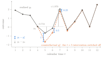
Two paths, one gap
The gap y_t-y^{c}_t: 1, 0.5, 0.25 at t=5,6,7. The change since y_4: -0.731, -0.197, 1.970.
Two clocks
Calendar time t dates the intervention and the regression row. Horizon h counts the periods after it.
| at t=5 |
5, 6, 7 |
0, 1, 2 |
1, 0.5, 0.25 |
| at t=10 |
10, 11, 12 |
0, 1, 2 |
1, 0.5, 0.25 |
Same gaps at different dates: the rule treats an intervention the same way whenever it arrives, so the response depends on h, not on t. The impulse-response function is h\mapsto\theta_h.
The 7.87-point rise was a calendar-time fact about 1950–1953. The policymaker asked a horizon question, and one regression will estimate one point on its curve.
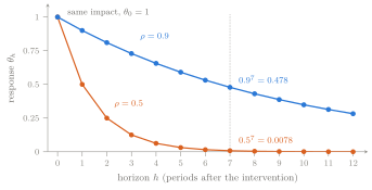
Persistence sets the shape
Iterate y_t=\rho\,y_{t-1}+\theta_0 s_t+v_t forward: \theta_h=\theta_0\rho^{h}.
The intervention sets only the first step; persistence does the rest. An AR(1) response can only decay.
The forward equation is a regression
\begin{aligned}
y_{t+h}&=\theta_0\rho^{h}\,s_t+\rho^{h+1}\,y_{t-1}+u_{t,h}\\
u_{t,h}&=\textstyle\sum_{j=0}^{h}\rho^{h-j}v_{t+j}+\theta_0\sum_{j=1}^{h}\rho^{h-j}s_{t+j}
\end{aligned}
u_{t,h} holds only terms dated t or later, and not s_t.
Interventions are unpredictable and independent of the disturbances (A2, A3), so u_{t,h} is uncorrelated with s_t and y_{t-1} and \beta_h=\theta_h. Least squares did none of that work.
One regression per horizon: a local projection. Without y_{t-1}, the same \beta_h but a noisier estimate (sd of \hat\beta_0 0.218, not 0.073).
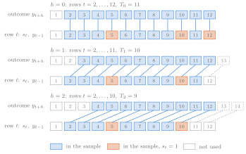
Rows by hand
T_h=T-h-p: 11, 10, 9 rows. Slopes 0.617, -0.983, 2.050 against \theta_h of 1, 0.5, 0.25.
One episode
With a single intervention row \tau:
\hat\beta_h=y_{\tau+h}-\bar y_{\text{others}}
The hand table with only the t=5 intervention, at h=0:
\hat\beta_0=-1.632=\underbrace{1}_{\theta_0}
+\underbrace{0.5\,y_4+v_5-\bar y_{\text{others}}}_{\text{everything else}\;=\;-2.632}
Korea is one such row. More episodes help only if what else happened is unrelated to the news.
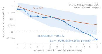
One draw against the truth
One T=200 sample: all estimates below \theta_h=0.9^h.
A caption names the intervention, the units of s and y, the horizon unit, and the counterfactual.
Inside the residual
\begin{aligned}
u_{t,1}&=\rho\,v_t+v_{t+1}+\theta_0s_{t+1}\\
u_{t+1,1}&=\rho\,v_{t+1}+v_{t+2}+\theta_0s_{t+2}
\end{aligned}
Adjacent rows share v_{t+1}: correlation \rho/(2+\rho^2). At horizon h, residuals up to h rows apart are correlated.
Across horizons, u_{t,h+1}=\rho\,u_{t,h}+v_{t+h+1}+\theta_0s_{t+h+1}.
Lecture 5 shows that inference depends on the autocorrelation of s_tu_{t,h}, which is zero here because s_t is independent of all the other terms and y_{t-1} is a control.
What has not yet been argued
| 1941Q4 |
0.6919 |
0.2612 |
0.2612 |
| 1950Q3 |
0.6001 |
0.1958 |
0.4570 |
| 1942Q3 |
0.4328 |
0.1009 |
0.5579 |
| 1950Q4 |
0.4022 |
0.0869 |
0.6448 |
Shares of \sum_t(s_t-\bar s)^2 in the h=8 sample of 496 quarters. Dropping 1950Q3 alone moves \hat\beta_8 from 0.362 to 0.434.
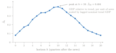
Still to argue: units (Lecture 2); controls, since Ramey and Zubairy’s set lowers \hat\beta_{10} to 0.294 (Lecture 3); identification (Lectures 3–4); uncertainty (Lectures 5–6); episode dependence (Lecture 13).
The Shock-to-Response Explorer
Open the Explorer; predict before touching a control.
- Two paths: switch off the t=5 intervention.
- Rows: move h and watch rows leave the sample.
- One draw: toggle y_{t-1} and shorten T.
- Military news: drop 1941Q4 or 1950Q3 at h=8.
Practicum 01 reruns these rows in Stata and reproduces the levels curve of Jordà–Taylor Figure 1a at a reduced draw count.
Exercises, hints, and worked solutions
- Start with the Lecture 01 exercises: six by hand, four in Stata, one of them on the military-news data.
- Open Hint only when you need a direction.
- Compare your work with the Detailed solution. Every Stata solution ends in assertions you can run.
The solutions companion also provides a printable PDF with all 10 hints and solutions expanded.
Next lecture
- Every regression here used the level y_{t+h}, with y_{t-1} on the right-hand side.
- The opening’s 7.87 points was a change, y_{t+h}-y_{t-1}, and a change since the date before is not a causal response.
If we regress y_{t+h}-y_{t-1} instead of y_{t+h}, is the answer different, or the same answer in different clothes?
Lecture 2: levels, differences, cumulative responses, and units, on the same military-news data.