P01 · The Instructor Build
Recover the Basic LP Estimator, executed in StataNow/SE 19.5
This is the executed version of Practicum 01. Every number and figure below was produced by master.do solution in the lab project, run in batch with StataNow/SE 19.5 on 2026-09-13; the logs are committed beside this page in output/. Stata does not run in the site build, so the outputs are static assets: rerun master.do to regenerate them.
REP01 is a statistical reproduction of Figure 1a of Jordà and Taylor (2025). It averages 500 of the 10,000 simulated draws behind the published curve (editor decision D2). At 500 draws it is exact: it matches the course benchmark and the authors’ own script to within 4\times10^{-8}. Against the published 10,000-draw means the match is statistical, and no horizon lies more than 1.71 Monte Carlo standard errors away. The data are simulated inside the authors’ script, so there is no data vintage; the problem set’s last task uses Ramey and Zubairy’s February 2018 package, fetched by a checksummed script and not redistributed. Before quoting a number, remember what the curve is: the average of an estimator over simulated samples, which lies below the true response 0.95^h at every horizon after impact. It is not an estimate from data, and it carries no standard error, because the authors’ code keeps none.
Expectations the outputs will test
Before the first run, the prior was:
- at 500 draws StataNow/SE 19.5 would return the Stata/SE 18.5 benchmark to every printed digit, as the planning run of the authors’ script had;
- course code written in the lecture’s notation, which stores each draw as a
doubleand records T_h frome(N), would differ from the authors’floatmeans only in the eighth decimal; - the 500-draw means would sit within about two Monte Carlo standard errors of the authors’ 10,000-draw means, with the largest gap near h=2, where the planning run found 0.018; and
- the sample handoff record’s Lab 4 hypothesis, a fall to about 0.30, would be refuted, because dropping 1950Q3 raises the h=8 estimate.
Written down, each of these can be contradicted by an output below.
How the build ran
cd practica/p01-question-to-projection/lab-project
/Applications/StataNow/StataSE.app/Contents/MacOS/stata-se -e do master.do solution| Item | Record |
|---|---|
| Software | StataNow/SE 19.5, batch mode, macOS |
| Started and finished | 13 Sep 2026 22:46:54; 13 Sep 2026 22:49:11 |
| Runtime | 137.1 seconds by Stata’s timer: the checks; REP01 in 63.7 s (Monte Carlo 15.1 s, authors’ script 46.4 s); the problem set in 72.3 s (its Monte Carlo 70.8 s); the handoff check |
| Draws | R=500 in REP01 and in Task 4 of the problem set (D2) |
| Checks | 200 assertions passed and none failed: 49 on the data and helpers, 65 in REP01, 48 in the problem set, 38 in the handoff check (assertions.csv) |
| Ramey–Zubairy data | Downloaded from the authors’ archive link and verified by data/raw/get_rz.do in the build’s first run; the final run found that copy and verified both checksums again |
| Logs | master.log, checks.log, rep01.log, pset.log, handoff-check.log, each written by log using inside its do-file |
The archive students download was rebuilt on 2026-09-14 with the solution inside it and run twice from fresh unzips in empty folders. With the defaults, do master.do passed 45 checks (the four on the Ramey–Zubairy workbook wait until Task 5 downloads it) and all 65 REP01 assertions at R=200, then stopped at the starter’s first check, FAIL Task 1: T_h = 11 - h at h = 0, 1, 2 (T = 12, p = 1), which is what an unwritten problem set should do. do master.do solution ran the solution at R=500, downloaded and verified the Ramey–Zubairy files, and ended in MASTER COMPLETE with 196 assertions passed and none failed: 45 checks, 65 REP01, 48 STA01, and 38 handoff. That run reproduced rep01-benchmark.csv, handoff-check.csv, both REP01 figures, both problem-set figures, the two caption files, not-yet-argued.txt, and sta01-news-shares.csv byte for byte from output/.
Three changes made on 2026-09-14 touch files this build had run, and none of them changes a command: the solution moved into lab-project/solution/ and into the archive (D54); header comments in rep01.do, starter/pset.do, solution/pset_solution.do, and handoff/check_handoff.do were revised for D54 and D55; and the two cap cd lines in each of the authors’ vendor/jel-code/ scripts, which named folders on their own machines, were commented out so that the archive holds no absolute path. The rerun above is the evidence that no number moved.
1. Replication REP01
The code that ran
replication/rep01.do, unabridged. lp_assert and lp_close come from helpers/lp_helpers.do: each runs Stata’s assert, prints pass or FAIL, records the result in output/assertions.csv, and stops the file on a failure; lp_close a b, tol(#) asserts that \lvert a-b\rvert is below the tolerance and prints both numbers.
*! rep01.do  REP01 . Recover the basic local-projection estimator
*
*  Local Projections: From First Principles to Empirical Research, Practicum 01.
*
*  Target   Jorda and Taylor (2025), "Local Projections," Journal of Economic
*           Literature 63(1), 59-110, Figure 1a: the Monte Carlo mean of the
*           levels local projection at h = 0,...,10, with an intercept and
*           without the lagged difference.
*  Package  ojorda/JEL-Code, commit 655696c1c576b7537c5a939d2c261f0a111ae663
*           (CC0), Example1_LongDifferences/SSBias_IntcpYLagdiffN_95.do,
*           shipped in vendor/jel-code/ with the authors' cap cd folder
*           paths commented out.
*  Kind     Statistical reproduction. The published figure averages 10,000
*           draws; this file averages $R draws (instructor build 500, student
*           default 200; editor decision D2). At a matched draw count the
*           reproduction is exact: every mean within 1e-6.
*  Mapping  vy = s_t (the intervention), e = v_t (the disturbance),
*           theta_0 = 1, rho = 0.95, T = 100 after 500 burn-in periods,
*           p = 1, so T_h = 99 - h.
*
*  Reads    replication/benchmark/REP01-levels-lp.csv          500 draws, Stata 18.5
*           replication/benchmark/REP01-author-R200-v195.csv   authors' script, 200 draws, StataNow 19.5
*           vendor/jel-code/SSBias_IntcpYLagdiffN_95.dta       authors' shipped means, 10,000 draws
*           vendor/jel-code/SSBias_IntcpYLagdiffN_95.do        run as shipped when AUTHOR_CHECK = 1
*  Writes   output/rep01.log, output/rep01-draws.dta, output/rep01-benchmark.csv,
*           output/fig-rep01-levels-mean.svg/.png, output/fig-rep01-first-draw.svg/.png
*  Globals  R             number of draws (default 200)
*           AUTHOR_CHECK  1 runs the authors' script at the same R (default 1)
*
*  Run from the lab project's top folder: do replication/rep01.do

version 19
clear
set more off
capture program list lp_assert
if _rc do helpers/lp_helpers.do
lp_root
capture mkdir output
capture log close rep01
log using "output/rep01.log", text replace name(rep01)
if "$R" == "" global R 200
if "$AUTHOR_CHECK" == "" global AUTHOR_CHECK 1
global LP_STEP rep01
local R = $R
confirm integer number `R'
timer clear 11
timer on 11
local npass0 = cond("$LP_NPASS" == "", 0, $LP_NPASS)

*==========================================================================
* 0. Settings, with the lines of SSBias_IntcpYLagdiffN_95.do they come from
*==========================================================================
local nobs = 100                  // all-simulate.do line 18
local burn = 500                  // line 20
local tobs = `nobs' + `burn'      // line 21
local hmax = 10                   // line 24
local rho  = 0.95                 // line 27
local seed = 12345                // line 39
display as text _n "REP01: levels LP, rho = `rho', T = `nobs', burn-in `burn', h = 0,...,`hmax', R = `R'"

*==========================================================================
* 1. One realization, one horizon: draw 1 of the authors' loop, rebuilt
*    outside the loop
*==========================================================================
clear
set seed `seed'
set obs `tobs'
generate t = _n
tsset t
generate vy = rnormal()           // line 52: the intervention s_t, drawn first
generate y  = 0                   // line 53: stored as float, as in the authors' code
generate e  = rnormal()           // line 56: the disturbance v_t, drawn second
* line 59 reads  y = $rho*l.y + $a*l.d.y + vy + e  if _n > 2,  with $a = 0.00 (line 57)
replace y = `rho'*L.y + vy + e if _n > 2
drop if _n <= `burn'              // line 62: keep the last 100 periods
replace t = _n
tsset t

regress F0.y vy L.y               // line 87 at h = 0
lp_assert "REP01 step 1: the h = 0 regression has T_0 = 99 rows" : e(N) == 99
lp_close _b[vy] 1.06035137, tol(1e-6) label(REP01 step 1: draw 1 at h = 0)

*==========================================================================
* 2. The same draw at every horizon: one regression per point of the curve
*==========================================================================
tempfile draw1
tempname D
postfile `D' h double b_draw1 T_draw1 using `draw1'
forvalues h = 0/`hmax' {
    quietly regress F`h'.y vy L.y
    post `D' (`h') (_b[vy]) (e(N))
}
postclose `D'
preserve
use `draw1', clear
format b_draw1 %12.8f
list, clean noobs
matrix input DRAW1 = (1.06035137, 0.99981713, 0.59646147, 0.55573124, 0.40316078, ///
    0.21355943, 0.08826523, -0.14803843, -0.28229347, -0.25071168, 0.24310037)
lp_assert "REP01 step 2: T_h = 99 - h in draw 1" : T_draw1 == 99 - h
forvalues h = 0/`hmax' {
    local i = `h' + 1
    lp_close b_draw1[`i'] DRAW1[1,`i'], tol(1e-6) label(REP01 step 2: draw 1 at h = `h')
}
restore

*==========================================================================
* 3. The Monte Carlo: R draws from one seeded stream (line 39), the levels
*    LP at h = 0,...,10 in each (lines 84-90)
*==========================================================================
display as text _n "Monte Carlo with R = `R' draws ..."
timer clear 12
timer on 12
tempname M
postfile `M' rep h double b T_h using "output/rep01-draws.dta", replace
set seed `seed'
quietly forvalues r = 1/`R' {
    clear
    set obs `tobs'
    generate t = _n
    tsset t
    generate vy = rnormal()
    generate y  = 0
    generate e  = rnormal()
    replace y = `rho'*L.y + vy + e if _n > 2
    drop if _n <= `burn'
    replace t = _n
    tsset t
    forvalues h = 0/`hmax' {
        regress F`h'.y vy L.y
        post `M' (`r') (`h') (_b[vy]) (e(N))
    }
}
postclose `M'
timer off 12
quietly timer list 12
local mc_seconds = r(t12)
display as text "Monte Carlo runtime: " as result %8.2f `mc_seconds' as text " seconds for R = `R'"

use "output/rep01-draws.dta", clear
lp_assert "REP01: every draw has T_h = 99 - h rows" : T_h == 99 - h
lp_assert "REP01: R draws at each of 11 horizons" : _N == 11*`R'

*--------------------------------------------------------------------------
* 4. Means over all R draws, and over the first 200 and 500 draws, which are
*    the matched counts of the two exact benchmarks
*--------------------------------------------------------------------------
preserve
collapse (mean) mean_R=b (sd) sd_R=b (p5) p5_R=b (p95) p95_R=b (count) draws=b, by(h)
tempfile summary
save `summary'
restore
foreach m in 200 500 {
    tempfile sum`m'
    preserve
    if `R' >= `m' {
        keep if rep <= `m'
        collapse (mean) mean_`m'=b, by(h)
    }
    else {
        keep if rep == 1
        keep h
        generate double mean_`m' = .
    }
    save `sum`m''
    restore
}

import delimited using "replication/benchmark/REP01-levels-lp.csv", clear varnames(1) encoding(utf8)
lp_assert "REP01 benchmark file: 11 rows of the levels series" : _N == 11 & series == "levels"
keep horizon coefficient true_response n
rename (horizon coefficient true_response n) (h published_500 published_theta published_T_h)
tempfile bench
save `bench'

import delimited using "replication/benchmark/REP01-author-R200-v195.csv", clear varnames(1)
rename (rl rt) (author_200 author_theta_200)
tempfile author200
save `author200'

use "vendor/jel-code/SSBias_IntcpYLagdiffN_95.dta", clear
keep t rl rt
rename (t rl rt) (h author_10000 author_theta)
tempfile author10000
save `author10000'

use `summary', clear
foreach f in sum200 sum500 bench author200 author10000 {
    merge 1:1 h using ``f'', nogenerate assert(match)
}
generate double theta_h = `rho'^h
generate T_h = 99 - h
generate double mcse_R = sd_R/sqrt(`R')
generate double diff_500 = mean_500 - published_500
generate double diff_200 = mean_200 - author_200
generate double se_10000 = sd_R*sqrt(1/`R' + 1/10000)
generate double z_10000 = (mean_R - author_10000)/se_10000
generate double se_500 = sd_R*sqrt(abs(1/`R' - 1/500))
generate double z_500 = cond(`R' == 500, 0, (mean_R - published_500)/se_500)

format theta_h published_500 mean_500 diff_500 author_200 mean_200 diff_200 author_10000 mean_R sd_R mcse_R %11.8f
format z_10000 z_500 %6.2f
display as text _n "REP01 comparison by horizon"
list h T_h theta_h published_500 mean_500 diff_500 author_200 mean_200 diff_200, clean noobs
list h author_10000 mean_R sd_R mcse_R z_10000 z_500, clean noobs

*--------------------------------------------------------------------------
* 5. Assertions against the benchmarks
*--------------------------------------------------------------------------
lp_assert "REP01: the benchmark's derived row count is T_h = 99 - h" : published_T_h == 99 - h
lp_assert "REP01: the true response equals the authors' rt (1e-6)" : abs(author_theta - theta_h) < 1e-6
lp_assert "REP01: the true response equals the benchmark's true_response (1e-6)" : abs(published_theta - theta_h) < 1e-6

if `R' >= 500 {
    forvalues h = 0/`hmax' {
        local i = `h' + 1
        lp_close mean_500[`i'] published_500[`i'], tol(1e-6) ///
            label(REP01 exact: first 500 draws against the published benchmark at h = `h')
    }
}
else display as text "Fewer than 500 draws: the exact comparison with the 500-draw benchmark is skipped."

if `R' >= 200 {
    forvalues h = 0/`hmax' {
        local i = `h' + 1
        lp_close mean_200[`i'] author_200[`i'], tol(1e-6) ///
            label(REP01 exact: first 200 draws against the authors' script at 200 draws at h = `h')
    }
}
else display as text "Fewer than 200 draws: the exact comparison with the 200-draw run is skipped."

* Statistical comparisons. The published figure's 10,000 draws are treated as
* an independent stream, which gives the wider of the two possible bounds.
forvalues h = 0/`hmax' {
    local i = `h' + 1
    local z = z_10000[`i']
    lp_assert "REP01 statistical: mean of `R' draws within 3 Monte Carlo SE of the 10,000-draw mean at h = `h' (z = `: display %5.2f `z'')" : abs(`z') < 3
}
if `R' != 500 {
    forvalues h = 0/`hmax' {
        local i = `h' + 1
        local z = z_500[`i']
        lp_assert "REP01 statistical: mean of `R' draws within 3 nested Monte Carlo SE of the 500-draw benchmark at h = `h' (z = `: display %5.2f `z'')" : abs(`z') < 3
    }
}
tempfile results
save `results'

*--------------------------------------------------------------------------
* 6. Cross-check: the authors' script at the same number of draws
*--------------------------------------------------------------------------
local author_seconds = .
if "$AUTHOR_CHECK" == "1" {
    save `results', replace
    local here = c(pwd)
    capture mkdir "output/rep01-author"
    quietly cd "output/rep01-author"
    global nobs = `nobs'
    global nreps = `R'
    display as text _n "Running vendor/jel-code/SSBias_IntcpYLagdiffN_95.do with nreps = `R' (progress counter follows)"
    timer clear 13
    timer on 13
    capture noisily quietly do "`here'/vendor/jel-code/SSBias_IntcpYLagdiffN_95.do"
    local rc = _rc
    timer off 13
    quietly cd "`here'"
    if `rc' {
        display as error "The authors' script stopped with r(`rc')."
        exit `rc'
    }
    quietly timer list 13
    local author_seconds = r(t13)
    display as text _n "Authors' script runtime: " as result %8.2f `author_seconds' as text " seconds"
    keep t rl rt
    rename (t rl rt) (h author_script_R author_script_theta)
    merge 1:1 h using `results', nogenerate assert(match)
    sort h
    forvalues h = 0/`hmax' {
        local i = `h' + 1
        lp_close author_script_R[`i'] mean_R[`i'], tol(1e-6) ///
            label(REP01 cross-check: authors' script against this file at R = `R' and h = `h')
    }
    lp_assert "REP01 cross-check: the authors' true response equals 0.95^h (1e-6)" : abs(author_script_theta - theta_h) < 1e-6
    macro drop nobs nreps burn tobs hmax rho a
}
else {
    display as text "AUTHOR_CHECK = 0: the authors' script was not run."
    generate double author_script_R = .
}
generate double diff_author = author_script_R - mean_R
sort h

*--------------------------------------------------------------------------
* 7. The benchmark record, one row per horizon
*--------------------------------------------------------------------------
tempname B
postfile `B' h T_h double(theta_h published_R500 reproduced_R500 diff_R500      ///
    author_R200_v195 reproduced_R200 diff_R200 author_R10000 reproduced_R      ///
    sd_R mcse_R z_vs_R10000 author_script diff_author_script) draws            ///
    double tolerance using "output/rep01-benchmark.dta", replace
forvalues i = 1/11 {
    post `B' (h[`i']) (T_h[`i']) (theta_h[`i']) (published_500[`i'])            ///
        (mean_500[`i']) (diff_500[`i']) (author_200[`i']) (mean_200[`i'])      ///
        (diff_200[`i']) (author_10000[`i']) (mean_R[`i']) (sd_R[`i'])          ///
        (mcse_R[`i']) (z_10000[`i']) (author_script_R[`i']) (diff_author[`i']) ///
        (`R') (1e-6)
}
postclose `B'
preserve
use "output/rep01-benchmark.dta", clear
format theta_h-diff_author_script %12.8f
export delimited using "output/rep01-benchmark.csv", replace datafmt
restore

*--------------------------------------------------------------------------
* 8. Figures
*--------------------------------------------------------------------------
set scheme stcolor
merge 1:1 h using `draw1', nogenerate assert(match)
local ink    "82 81 78"
local muted  "137 135 129"
local blue   "42 120 214"
local orange "217 96 31"
local rule   "195 194 183"

twoway (line theta_h h, lcolor("`ink'") lwidth(medthick))                              ///
       (line author_10000 h, lcolor("`muted'") lpattern(dash) lwidth(medium))          ///
       (scatter published_500 h, msymbol(Oh) mcolor("`orange'") msize(large) mlwidth(medthick)) ///
       (connected mean_R h, lcolor("`blue'") mcolor("`blue'") msymbol(O) msize(small) lwidth(medthick)), ///
       xlabel(0(1)10, nogrid)                                                          ///
       ylabel(0.4(0.1)1.0, format(%3.1f) angle(0) glcolor("`rule'") glpattern(solid) glwidth(vthin)) ///
       xtitle("Horizon h (periods after the intervention)")                            ///
       ytitle("Mean of the estimate across draws")                                     ///
       legend(order(1 "True response 0.95{sup:h}"                                      ///
                    2 "Authors' shipped mean, 10,000 draws"                            ///
                    3 "Course benchmark, 500 draws (Stata 18.5)"                       ///
                    4 "This run, `R' draws (StataNow 19.5)")                           ///
              cols(1) position(1) ring(0) region(lstyle(none) fcolor(white)) size(small)) ///
       graphregion(color(white)) plotregion(color(white)) xsize(6.5) ysize(4.2)
graph export "output/fig-rep01-levels-mean.svg", replace
graph export "output/fig-rep01-levels-mean.png", replace width(1950)

twoway (rarea p5_R p95_R h, color("`blue'%15") lwidth(none))                           ///
       (line theta_h h, lcolor("`ink'") lwidth(medthick))                              ///
       (connected mean_R h, lcolor("`blue'") mcolor("`blue'") msymbol(O) msize(small) lwidth(medthick)) ///
       (connected b_draw1 h, lcolor("`orange'") mcolor("`orange'") msymbol(D) msize(small) lwidth(medium)), ///
       yline(0, lcolor("`rule'")) xlabel(0(1)10, nogrid)                               ///
       ylabel(-0.4(0.2)1.4, format(%3.1f) angle(0) glcolor("`rule'") glpattern(solid) glwidth(vthin)) ///
       xtitle("Horizon h (periods after the intervention)")                            ///
       ytitle("Estimate (units of y per unit of s)")                                   ///
       legend(order(2 "True response 0.95{sup:h}" 3 "Mean of `R' draws"                ///
                    4 "Draw 1 (seed 12345)" 1 "Middle 90 percent of the `R' draws")    ///
              cols(2) position(6) region(lstyle(none)) size(small))                    ///
       graphregion(color(white)) plotregion(color(white)) xsize(6.5) ysize(4.4)
graph export "output/fig-rep01-first-draw.svg", replace
graph export "output/fig-rep01-first-draw.png", replace width(1950)

*--------------------------------------------------------------------------
timer off 11
quietly timer list 11
local total_seconds = r(t11)
local npass = $LP_NPASS - `npass0'
display as text _n "REP01 complete: " as result `npass' as text " assertions passed; R = `R'; Monte Carlo " ///
    as result %7.2f `mc_seconds' as text " s; authors' script " as result %7.2f `author_seconds' ///
    as text " s; total " as result %7.2f `total_seconds' as text " s"
log close rep01
The first draw
Log excerpt from rep01.log, unabridged for the target numbers:
. regress F0.y vy L.y               // line 87 at h = 0

      Source |       SS           df       MS      Number of obs   =        99
-------------+----------------------------------   F(2, 96)        =    251.99
       Model |  501.423656         2  250.711828   Prob > F        =    0.0000
    Residual |  95.5114248        96  .994910675   R-squared       =    0.8400
-------------+----------------------------------   Adj R-squared   =    0.8367
       Total |   596.93508        98  6.09117429   Root MSE        =    .99745

------------------------------------------------------------------------------
           y | Coefficient  Std. err.      t    P>|t|     [95% conf. interval]
-------------+----------------------------------------------------------------
          vy |   1.060351   .1026716    10.33   0.000     .8565499    1.264153
             |
           y |
         L1. |    .909107   .0428413    21.22   0.000     .8240676    .9941464
             |
       _cons |   .1509078   .1147404     1.32   0.192    -.0768501    .3786656
------------------------------------------------------------------------------

. lp_assert "REP01 step 1: the h = 0 regression has T_0 = 99 rows" : e(N) == 99
pass  REP01 step 1: the h = 0 regression has T_0 = 99 rows

. lp_close _b[vy] 1.06035137, tol(1e-6) label(REP01 step 1: draw 1 at h = 0)
REP01 step 1: draw 1 at h = 0
      value      1.06035143   target      1.06035137   |diff|  5.95e-08   tol  1.0e-06
pass  REP01 step 1: draw 1 at h = 0

. list, clean noobs

     h       b_draw1   T_draw1
     0    1.06035143        99
     1    0.99981716        98
     2    0.59646150        97
     3    0.55573121        96
     4    0.40316077        95
     5    0.21355944        94
     6    0.08826523        93
     7   -0.14803844        92
     8   -0.28229347        91
     9   -0.25071169        90
    10    0.24310038        89
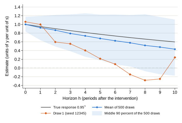
The first draw’s impact estimate is 1.06035143 on 99 rows. The check’s target, 1.06035137, is the same coefficient as the authors’ float variable stores it, 6\times10^{-8} away: display %11.8f float(_b[vy]) prints it after the regression, and the eleven values of DRAW1 are this draw’s coefficients under the same storage. Across horizons the draw falls from 1.060 to −0.282 at h=8 and is back at 0.243 at h=10, while 0.95^h never falls below 0.599.
The comparison with the benchmarks
. display as text _n "REP01 comparison by horizon"

REP01 comparison by horizon

. list h T_h theta_h published_500 mean_500 diff_500 author_200 mean_200 diff_200, clean noobs

     h   T_h      theta_h   publis~500     mean_500      diff_500   author_200     mean_200      diff_200
     0    99   1.00000000   1.00175750   1.00175746   -0.00000004   0.99686521   0.99686519   -0.00000003
     1    98   0.95000000   0.92489529   0.92489526   -0.00000002   0.91357774   0.91357771   -0.00000003
     2    97   0.90250000   0.86787397   0.86787396   -0.00000001   0.85901380   0.85901381    0.00000002
     3    96   0.85737500   0.79257834   0.79257836    0.00000002   0.78925842   0.78925840   -0.00000002
     4    95   0.81450625   0.73754936   0.73754938    0.00000002   0.74316418   0.74316419    0.00000000
     5    94   0.77378094   0.67800373   0.67800374    0.00000001   0.68870902   0.68870901   -0.00000001
     6    93   0.73509189   0.62550861   0.62550860   -0.00000000   0.62830913   0.62830915    0.00000002
     7    92   0.69833730   0.57830870   0.57830868   -0.00000002   0.57235688   0.57235686   -0.00000002
     8    91   0.66342043   0.51882571   0.51882570   -0.00000001   0.50967115   0.50967116    0.00000001
     9    90   0.63024941   0.48049915   0.48049915    0.00000000   0.48197576   0.48197576    0.00000000
    10    89   0.59873694   0.43152007   0.43152008    0.00000001   0.42771590   0.42771590   -0.00000000

. list h author_10000 mean_R sd_R mcse_R z_10000 z_500, clean noobs

     h   auth~10000       mean_R         sd_R       mcse_R   z_10000   z_500
     0   0.99697095   1.00175746   0.10465395   0.00468027      1.00    0.00
     1   0.92157829   0.92489526   0.17283519   0.00772942      0.42    0.00
     2   0.84994626   0.86787396   0.22938530   0.01025842      1.71    0.00
     3   0.78295529   0.79257836   0.26442179   0.01182530      0.79    0.00
     4   0.72164255   0.73754938   0.30159171   0.01348759      1.15    0.00
     5   0.66630644   0.67800374   0.33255860   0.01487247      0.77    0.00
     6   0.61206740   0.62550860   0.35454376   0.01585568      0.83    0.00
     7   0.56319672   0.57830868   0.37134603   0.01660710      0.89    0.00
     8   0.51815391   0.51882570   0.39521070   0.01767436      0.04    0.00
     9   0.47492251   0.48049915   0.39662619   0.01773766      0.31    0.00
    10   0.42890212   0.43152008   0.39692485   0.01775102      0.14    0.00

REP01 complete: 65 assertions passed; R = 500; Monte Carlo   15.10 s; authors' script   46.39 s; total   63.71 s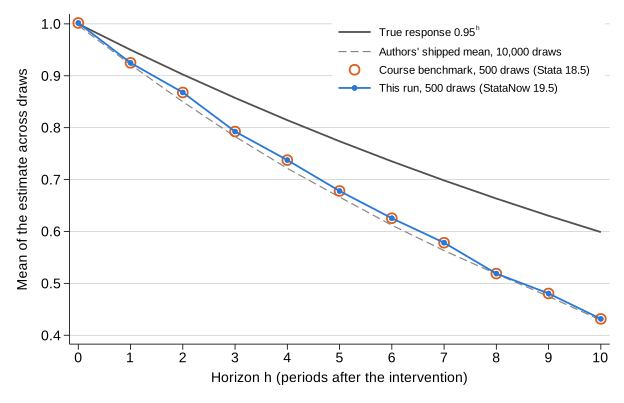
Benchmark comparison
All values are means of \hat\beta_h across draws, in units of y per unit of s; the published and author columns come from the authors’ script, the reproduced columns from rep01.do. The tolerance is 10^{-6} where the draw counts match and \lvert z\rvert<3 against the 10,000-draw means. The full record is rep01-benchmark.csv. Both benchmark files are read with the import delimited lines shown in rep01.do above; they print the same eight decimals with asdouble, and each difference column is formed against them as imported.
| h | \theta_h | Published, 500 draws, Stata 18.5 | Reproduced, 500 draws | Difference | Authors’ script, 500 draws, StataNow 19.5 | Authors’ script, 200 draws, StataNow 19.5 | Reproduced, first 200 draws | Difference | Authors’ shipped mean, 10,000 draws | z |
|---|---|---|---|---|---|---|---|---|---|---|
| 0 | 1.0000 | 1.00175750 | 1.00175746 | −0.00000004 | 1.00175750 | 0.99686521 | 0.99686519 | −0.00000003 | 0.99697095 | 1.00 |
| 1 | 0.9500 | 0.92489529 | 0.92489526 | −0.00000002 | 0.92489529 | 0.91357774 | 0.91357771 | −0.00000003 | 0.92157829 | 0.42 |
| 2 | 0.9025 | 0.86787397 | 0.86787396 | −0.00000001 | 0.86787397 | 0.85901380 | 0.85901381 | 0.00000002 | 0.84994626 | 1.71 |
| 3 | 0.8574 | 0.79257834 | 0.79257836 | 0.00000002 | 0.79257834 | 0.78925842 | 0.78925840 | −0.00000002 | 0.78295529 | 0.79 |
| 4 | 0.8145 | 0.73754936 | 0.73754938 | 0.00000002 | 0.73754936 | 0.74316418 | 0.74316419 | 0.00000000 | 0.72164255 | 1.15 |
| 5 | 0.7738 | 0.67800373 | 0.67800374 | 0.00000001 | 0.67800373 | 0.68870902 | 0.68870901 | −0.00000001 | 0.66630644 | 0.77 |
| 6 | 0.7351 | 0.62550861 | 0.62550860 | 0.00000000 | 0.62550861 | 0.62830913 | 0.62830915 | 0.00000002 | 0.61206740 | 0.83 |
| 7 | 0.6983 | 0.57830870 | 0.57830868 | −0.00000002 | 0.57830870 | 0.57235688 | 0.57235686 | −0.00000002 | 0.56319672 | 0.89 |
| 8 | 0.6634 | 0.51882571 | 0.51882570 | −0.00000001 | 0.51882571 | 0.50967115 | 0.50967116 | 0.00000001 | 0.51815391 | 0.04 |
| 9 | 0.6302 | 0.48049915 | 0.48049915 | 0.00000000 | 0.48049915 | 0.48197576 | 0.48197576 | 0.00000000 | 0.47492251 | 0.31 |
| 10 | 0.5987 | 0.43152007 | 0.43152008 | 0.00000001 | 0.43152007 | 0.42771590 | 0.42771590 | 0.00000000 | 0.42890212 | 0.14 |
Read the result. Where the draw counts match, the reproduction is exact: the largest absolute difference is 4e-8 at 500 draws and 3e-8 at 200 draws, and the authors’ unchanged script, rerun in StataNow/SE 19.5 at 500 draws, differs from rep01.do by at most 4e-8 while matching the Stata/SE 18.5 benchmark to every printed digit. Expectations 1 and 2 hold, and there is no software row for D1. Against the 10,000-draw means the largest z is 1.71, at h=2, where the gap is 0.0179, so expectation 3 holds as well. What the table does not show as a difference is the gap to the truth: the mean lies below \theta_h at every horizon from h=1 on, by 0.025 at h=1 and 0.167 at h=10, where the Monte Carlo standard error is 0.018. That gap belongs to the estimator in 100-period samples with \rho=0.95, and Lecture 2 takes it up.
The 65 checks REP01 passed, in order:
pass  REP01 step 1: the h = 0 regression has T_0 = 99 rows
pass  REP01 step 1: draw 1 at h = 0
pass  REP01 step 2: T_h = 99 - h in draw 1
pass  REP01 step 2: draw 1 at h = 0
pass  REP01 step 2: draw 1 at h = 1
pass  REP01 step 2: draw 1 at h = 2
pass  REP01 step 2: draw 1 at h = 3
pass  REP01 step 2: draw 1 at h = 4
pass  REP01 step 2: draw 1 at h = 5
pass  REP01 step 2: draw 1 at h = 6
pass  REP01 step 2: draw 1 at h = 7
pass  REP01 step 2: draw 1 at h = 8
pass  REP01 step 2: draw 1 at h = 9
pass  REP01 step 2: draw 1 at h = 10
pass  REP01: every draw has T_h = 99 - h rows
pass  REP01: R draws at each of 11 horizons
pass  REP01 benchmark file: 11 rows of the levels series
pass  REP01: the benchmark's derived row count is T_h = 99 - h
pass  REP01: the true response equals the authors' rt (1e-6)
pass  REP01: the true response equals the benchmark's true_response (1e-6)
pass  REP01 exact: first 500 draws against the published benchmark at h = 0
pass  REP01 exact: first 500 draws against the published benchmark at h = 1
pass  REP01 exact: first 500 draws against the published benchmark at h = 2
pass  REP01 exact: first 500 draws against the published benchmark at h = 3
pass  REP01 exact: first 500 draws against the published benchmark at h = 4
pass  REP01 exact: first 500 draws against the published benchmark at h = 5
pass  REP01 exact: first 500 draws against the published benchmark at h = 6
pass  REP01 exact: first 500 draws against the published benchmark at h = 7
pass  REP01 exact: first 500 draws against the published benchmark at h = 8
pass  REP01 exact: first 500 draws against the published benchmark at h = 9
pass  REP01 exact: first 500 draws against the published benchmark at h = 10
pass  REP01 exact: first 200 draws against the authors' script at 200 draws at h = 0
pass  REP01 exact: first 200 draws against the authors' script at 200 draws at h = 1
pass  REP01 exact: first 200 draws against the authors' script at 200 draws at h = 2
pass  REP01 exact: first 200 draws against the authors' script at 200 draws at h = 3
pass  REP01 exact: first 200 draws against the authors' script at 200 draws at h = 4
pass  REP01 exact: first 200 draws against the authors' script at 200 draws at h = 5
pass  REP01 exact: first 200 draws against the authors' script at 200 draws at h = 6
pass  REP01 exact: first 200 draws against the authors' script at 200 draws at h = 7
pass  REP01 exact: first 200 draws against the authors' script at 200 draws at h = 8
pass  REP01 exact: first 200 draws against the authors' script at 200 draws at h = 9
pass  REP01 exact: first 200 draws against the authors' script at 200 draws at h = 10
pass  REP01 statistical: mean of 500 draws within 3 Monte Carlo SE of the 10,000-draw mean at h = 0 (z =  1.00)
pass  REP01 statistical: mean of 500 draws within 3 Monte Carlo SE of the 10,000-draw mean at h = 1 (z =  0.42)
pass  REP01 statistical: mean of 500 draws within 3 Monte Carlo SE of the 10,000-draw mean at h = 2 (z =  1.71)
pass  REP01 statistical: mean of 500 draws within 3 Monte Carlo SE of the 10,000-draw mean at h = 3 (z =  0.79)
pass  REP01 statistical: mean of 500 draws within 3 Monte Carlo SE of the 10,000-draw mean at h = 4 (z =  1.15)
pass  REP01 statistical: mean of 500 draws within 3 Monte Carlo SE of the 10,000-draw mean at h = 5 (z =  0.77)
pass  REP01 statistical: mean of 500 draws within 3 Monte Carlo SE of the 10,000-draw mean at h = 6 (z =  0.83)
pass  REP01 statistical: mean of 500 draws within 3 Monte Carlo SE of the 10,000-draw mean at h = 7 (z =  0.89)
pass  REP01 statistical: mean of 500 draws within 3 Monte Carlo SE of the 10,000-draw mean at h = 8 (z =  0.04)
pass  REP01 statistical: mean of 500 draws within 3 Monte Carlo SE of the 10,000-draw mean at h = 9 (z =  0.31)
pass  REP01 statistical: mean of 500 draws within 3 Monte Carlo SE of the 10,000-draw mean at h = 10 (z =  0.14)
pass  REP01 cross-check: authors' script against this file at R = 500 and h = 0
pass  REP01 cross-check: authors' script against this file at R = 500 and h = 1
pass  REP01 cross-check: authors' script against this file at R = 500 and h = 2
pass  REP01 cross-check: authors' script against this file at R = 500 and h = 3
pass  REP01 cross-check: authors' script against this file at R = 500 and h = 4
pass  REP01 cross-check: authors' script against this file at R = 500 and h = 5
pass  REP01 cross-check: authors' script against this file at R = 500 and h = 6
pass  REP01 cross-check: authors' script against this file at R = 500 and h = 7
pass  REP01 cross-check: authors' script against this file at R = 500 and h = 8
pass  REP01 cross-check: authors' script against this file at R = 500 and h = 9
pass  REP01 cross-check: authors' script against this file at R = 500 and h = 10
pass  REP01 cross-check: the authors' true response equals 0.95^h (1e-6)
2. Problem set STA01, solved
solution/pset_solution.do ships inside the lab project (editor decision D54). Attempt the five tasks in starter/pset.do first: the checks tell you whether your own code is right, and the solution is worth reading only against an answer you have already tried to write.
In this build master.do solution ran the file at R=500. Its log is pset.log, the figures and written answers it exported are beside it in output/, and the checks it passed are the sta01 rows of assertions.csv. Each task below gives the code as it ran, the lines of pset.log that report the result (... marks omitted lines), a reading, and the checks. The file’s header comments were revised on 2026-09-14, when the solution moved into the archive; no command changed.
STA01 complete: 48 assertions passed in 72.3 seconds (R = 500).Two of those 48 checks belong to R=500: at the student default of 200 draws Task 4’s R=500 comparisons do not run and the file passes 46. The caption and paragraph checks confirm only that each slot holds a sentence of its own; the grading notes at the end of this section say how a reader marks what the sentences say.
The file opens with the setup lines of starter/pset.do.
version 19
clear
set more off
capture program list lp_assert
if _rc do helpers/lp_helpers.do
lp_root
capture mkdir output
capture mkdir output/pset
capture log close pset
log using "output/pset/pset.log", text replace name(pset)
if "$R" == "" global R 200
global LP_STEP sta01
local R = $R
confirm integer number `R'
local npass0 = cond("$LP_NPASS" == "", 0, $LP_NPASS)
set scheme stcolor
timer clear 21
timer on 21
local ink    "82 81 78"
local blue   "42 120 214"
local orange "217 96 31"
local rule   "195 194 183"
Task 1 · Construct the rows for h=0,1,2
For each horizon, the lead y_{t+h}, the rows with t\ge2 and a lead that exists, and their counts, without running a regression. Tasks 1 and 2 read the Explorer’s own export, handoff/hand_table.csv, because its SHA-256 equals the shipped data/raw/hand_table.csv.
*==========================================================================
* TASK 1 . Construct the rows for h = 0, 1, 2              (Exercise 3; Lab 2)
*==========================================================================
local handfile "data/raw/hand_table.csv"
capture confirm file "handoff/hand_table.csv"
if _rc == 0 {
    lp_sha256 "handoff/hand_table.csv"
    local sha_handoff "`r(sha256)'"
    lp_sha256 "data/raw/hand_table.csv"
    if "`sha_handoff'" == "`r(sha256)'" local handfile "handoff/hand_table.csv"
    else display as error "handoff/hand_table.csv differs from data/raw/hand_table.csv; Tasks 1-2 read data/raw."
}
display as text "Tasks 1 and 2 read `handfile'"
import delimited using "`handfile'", clear
tsset t

tempname H
postfile `H' h T_h n1 n0 first last using "output/pset/results_hand.dta", replace
forvalues h = 0/2 {
    generate double yh = F`h'.y
    generate byte inrow = (t >= 2 & yh < .)
    quietly count if inrow
    local T_h = r(N)
    quietly count if inrow & s == 1
    local n1 = r(N)
    quietly count if inrow & s == 0
    local n0 = r(N)
    quietly summarize t if inrow
    local first = r(min)
    local last  = r(max)
    display as text _n "h = `h': rows `first'-`last'"
    list t s y yh if inrow, clean noobs
    post `H' (`h') (`T_h') (`n1') (`n0') (`first') (`last')
    drop yh inrow
}
postclose `H'

use "output/pset/results_hand.dta", clear
list, clean noobs
lp_assert "Task 1: T_h = 11 - h at h = 0, 1, 2 (T = 12, p = 1)" : T_h == 11 - h
lp_assert "Task 1: every row is an intervention row or a comparison row" : n1 + n0 == T_h
lp_assert "Task 1: the rows run from t = 2 to t = 12 - h" : first == 2 & last == 12 - h
lp_assert "Task 1: 3 intervention rows at h = 0 and 2 at h = 1 and h = 2" : n1 == cond(h == 0, 3, 2)
Output.
. display as text "Tasks 1 and 2 read `handfile'"
Tasks 1 and 2 read handoff/hand_table.csv
...
h = 1: rows 2-11

     t   s           y           yh
     2   0        1.45        1.325
     3   0       1.325    .06249999
     4   0       .0625   -.66875005
     5   1     -.66875   -.13437502
     6   0    -.134375    2.0328124
     7   0    2.032812   -.28359374
     8   0   -.2835937    .65820313
     9   0    .6582031    1.9291016
    10   1    1.929102    .06455082
    11   0    .0645508    2.5322754
...
. list, clean noobs

    h   T_h   n1   n0   first   last
    0    11    3    8       2     12
    1    10    2    8       2     11
    2     9    2    7       2     10
Read the result. Each horizon costs the last row, and row 1 never enters because y_0 is not data, so T_h=11-h over the rows t=2 to t=12-h. The intervention in row 12 leaves first: at h=1 the rows stop at 11, the intervention rows fall from three to two, and the eight comparison rows are still there. At h=2 row 11 leaves as well, and because it is a comparison row n_0 falls to seven. Three horizons, three different sets of rows, and the counts say which rows carry the intervention before any slope is computed.
Checks.
pass  Task 1: T_h = 11 - h at h = 0, 1, 2 (T = 12, p = 1)
pass  Task 1: every row is an intervention row or a comparison row
pass  Task 1: the rows run from t = 2 to t = 12 - h
pass  Task 1: 3 intervention rows at h = 0 and 2 at h = 1 and h = 2
Task 2 · Estimate the slopes from the rows
The group means on those rows, the slope by hand as \sum_t(s_t-\bar s)\,y_{t+h}/\sum_t(s_t-\bar s)^2, the same slope from regress, and the slope with y_{t-1} added on the same rows.
*==========================================================================
* TASK 2 . Estimate the slopes from the rows                (Exercises 3-4)
*==========================================================================
import delimited using "`handfile'", clear
tsset t
tempname E
postfile `E' h double(ybar1 ybar0 b_hand b_reg b_ctrl) byte same_rows ///
    using "output/pset/results_hand_slopes.dta", replace
forvalues h = 0/2 {
    generate double yh = F`h'.y
    generate byte inrow = (t >= 2 & yh < .)

    quietly summarize yh if inrow & s == 1
    local ybar1 = r(mean)
    quietly summarize yh if inrow & s == 0
    local ybar0 = r(mean)

    quietly summarize s if inrow
    local sbar = r(mean)
    generate double num = (s - `sbar')*yh if inrow
    generate double den = (s - `sbar')^2 if inrow
    quietly summarize num
    local sum_num = r(sum)
    quietly summarize den
    local b_hand = `sum_num'/r(sum)

    quietly regress F`h'.y s if t >= 2
    local b_reg = _b[s]
    quietly count if e(sample) != inrow
    local mismatch = r(N)
    quietly regress F`h'.y s L.y if t >= 2
    local b_ctrl = _b[s]
    quietly count if e(sample) != inrow
    local same_rows = (`mismatch' + r(N) == 0)

    post `E' (`h') (`ybar1') (`ybar0') (`b_hand') (`b_reg') (`b_ctrl') (`same_rows')
    drop yh inrow num den
}
postclose `E'

use "output/pset/results_hand_slopes.dta", clear
merge 1:1 h using "output/pset/results_hand.dta", nogenerate assert(match)
save "output/pset/results_hand.dta", replace
format ybar1 ybar0 b_hand b_reg b_ctrl %12.8f
list h T_h ybar1 ybar0 b_hand b_reg b_ctrl same_rows, clean noobs
lp_assert "Task 2: the slope by hand equals the difference in means (1e-6)" : abs(b_hand - (ybar1 - ybar0)) < 1e-6
lp_assert "Task 2: regress returns the slope computed by hand (1e-6)" : abs(b_reg - b_hand) < 1e-6
lp_assert "Task 2: the regressions with and without y_(t-1) use the same rows" : same_rows == 1
lp_assert "Task 2: slopes without the control 0.617322, -0.983356, 2.050024 (1e-6)" : ///
    abs(b_reg - cond(h == 0, 0.617322, cond(h == 1, -0.983356, 2.050024))) < 1e-6
lp_assert "Task 2: slopes with y_(t-1) 0.575667, -1.050405, 2.153022 (1e-6)" : ///
    abs(b_ctrl - cond(h == 0, 0.575667, cond(h == 1, -1.050405, 2.153022))) < 1e-6
Output.
. list h T_h ybar1 ybar0 b_hand b_reg b_ctrl same_rows, clean noobs

    h   T_h         ybar1        ybar0        b_hand         b_reg        b_ctrl   same_r~s
    0    11    1.26420899   0.64688720    0.61732179    0.61732179    0.57566744          1
    1    10   -0.03491210   0.94844359   -0.98335570   -0.98335570   -1.05040516          1
    2     9    2.28254390   0.23251953    2.05002437    2.05002437    2.15302240          1
Read the result. With a 0–1 intervention the slope without a control is the difference in group means: at h=0 it is 1.26420899-0.64688720=0.61732179, and the hand calculation and regress return it to every printed digit. Adding y_{t-1} on the same rows moves the slopes to 0.575667, −1.050405, and 2.153022. They are no longer differences in means, and none of the six is near \theta_h=0.5^h, which is 1, 0.5, and 0.25: with three intervention rows, and then two, a single disturbance moves a slope further than the response itself does. same_rows records that both regressions used exactly the rows of Task 1, which is what makes the comparison a controlled one. The eighth decimals are those of import delimited, which stores v and y as float; every check compares at 10^{-6}.
Checks.
pass  Task 2: the slope by hand equals the difference in means (1e-6)
pass  Task 2: regress returns the slope computed by hand (1e-6)
pass  Task 2: the regressions with and without y_(t-1) use the same rows
pass  Task 2: slopes without the control 0.617322, -0.983356, 2.050024 (1e-6)
pass  Task 2: slopes with y_(t-1) 0.575667, -1.050405, 2.153022 (1e-6)
Task 3 · A response in a loop
Thirteen regressions on the T=200 seed-2 sample that Lab 3 displays, each posting the coefficient on s_t with its e(N).
*==========================================================================
* TASK 3 . A response in a loop                            (Exercise 6; Lab 3)
*==========================================================================
local drawfile "data/raw/onedraw_rho09_seed2.csv"
capture confirm file "handoff/onedraw_rho09_seed2.csv"
if _rc == 0 {
    import delimited using "handoff/onedraw_rho09_seed2.csv", clear
    rename (s v y) (s_b v_b y_b)
    tempfile browser
    save `browser'
    import delimited using "data/raw/onedraw_rho09_seed2.csv", clear
    merge 1:1 t using `browser', nogenerate
    quietly count if missing(s_b) | abs(s - s_b) > 1e-7 | abs(v - v_b) > 1e-7 | abs(y - y_b) > 1e-7
    if r(N) == 0 local drawfile "handoff/onedraw_rho09_seed2.csv"
    else display as error "handoff/onedraw_rho09_seed2.csv differs from the shipped draw; Task 3 reads data/raw."
}
display as text "Task 3 reads `drawfile'"
import delimited using "`drawfile'", clear
tsset t
lp_assert "Task 3: the draw holds T = 200 periods" : _N == 200

tempname P
postfile `P' h double beta_h T_h using "output/pset/results_onedraw.dta", replace
forvalues h = 0/12 {
    quietly regress F`h'.y s L.y
    post `P' (`h') (_b[s]) (e(N))
}
postclose `P'

use "output/pset/results_onedraw.dta", clear
generate double theta_h = 0.9^h
format beta_h theta_h %9.6f
list, clean noobs
lp_assert "Task 3: T_h = 199 - h at every horizon" : T_h == 199 - h
lp_close beta_h[1] 0.878940, tol(1e-6) label(Task 3: beta_0 = 0.878940)
lp_close beta_h[13] -0.293297, tol(1e-6) label(Task 3: beta_12 = -0.293297)
quietly count if beta_h < theta_h
local below = r(N)
lp_assert "Task 3: the estimate lies below theta_h at all 13 horizons" : `below' == 13
save "output/pset/results_onedraw.dta", replace
Output.
. display as text "Task 3 reads `drawfile'"
Task 3 reads handoff/onedraw_rho09_seed2.csv
...
. list, clean noobs

     h      beta_h   T_h    theta_h
     0    0.878940   199   1.000000
     1    0.853260   198   0.900000
     2    0.612737   197   0.810000
     3    0.611046   196   0.729000
     4    0.548477   195   0.656100
     5    0.583099   194   0.590490
     6    0.509120   193   0.531441
     7    0.417788   192   0.478297
     8    0.240595   191   0.430467
     9    0.130293   190   0.387420
    10   -0.028821   189   0.348678
    11   -0.117200   188   0.313811
    12   -0.293297   187   0.282430
Read the result. T_h=199-h at every horizon, and all thirteen estimates lie below \theta_h=0.9^h: 0.878940 against 1 at impact, 0.583099 against 0.590490 at h=5, and −0.293297 against 0.282430 at h=12. Read on its own, the estimated response turns negative at h=10 and stays there, which the economy that produced the sample never does. Neighbouring regressions use almost the same rows and their residuals share terms (Lecture 01), so this is one sample’s error seen thirteen times rather than thirteen independent misses.
Checks.
pass  Task 3: the draw holds T = 200 periods
pass  Task 3: T_h = 199 - h at every horizon
      value      0.87894028   target      0.87894000   |diff|  2.81e-07   tol  1.0e-06
pass  Task 3: beta_0 = 0.878940
      value     -0.29329663   target     -0.29329700   |diff|  3.66e-07   tol  1.0e-06
pass  Task 3: beta_12 = -0.293297
pass  Task 3: the estimate lies below theta_h at all 13 horizons
Task 4 · Many draws, one graph, a caption with four slots
Seed 3 set once for each \rho, samples of 300 periods with all of s drawn before any v, the first 100 dropped, and at each horizon the slope with and without y_{t-1}; then the two summaries, the graph, and the caption.
*==========================================================================
* TASK 4 . Many draws, then the response graph and its caption   (Exercises 6-7)
*==========================================================================
display as text _n "Monte Carlo: R = `R' samples for each rho"
timer clear 22
timer on 22
tempname MC
postfile `MC' rep double rho h double(b_ctrl b_noctrl) n_ctrl n_noctrl ///
    using "output/pset/mc_draws.dta", replace
foreach rho in 0.5 0.9 {
    set seed 3                                   // once for each rho, outside the loop
    quietly forvalues r = 1/`R' {
        clear
        set obs 300
        generate t = _n
        tsset t
        generate s = rnormal()                   // all of s first,
        generate v = rnormal()                   // then all of v
        generate y = .
        replace y = s + v in 1                   // y_0 = 0
        replace y = `rho'*L.y + s + v in 2/300
        drop if t <= 100                         // burn-in of 100 periods
        replace t = _n
        tsset t
        forvalues h = 0/12 {
            regress F`h'.y s L.y
            local b_c = _b[s]
            local n_c = e(N)
            regress F`h'.y s
            post `MC' (`r') (`rho') (`h') (`b_c') (_b[s]) (`n_c') (e(N))
        }
    }
}
postclose `MC'
timer off 22
quietly timer list 22
display as text "Monte Carlo runtime: " as result %7.2f r(t22) as text " seconds for R = `R'"

use "output/pset/mc_draws.dta", clear
lp_assert "Task 4: 199 - h rows with the control and 200 - h without" : n_ctrl == 199 - h & n_noctrl == 200 - h
foreach m in 200 500 {
    if `R' >= `m' {
        preserve
        keep if rep <= `m'
        generate double theta_h = rho^h
        collapse (mean) theta_h mean_ctrl=b_ctrl mean_noctrl=b_noctrl      ///
                 (sd) sd_ctrl=b_ctrl sd_noctrl=b_noctrl                    ///
                 (p5) p5=b_ctrl (p95) p95=b_ctrl, by(rho h)
        generate double bias = mean_ctrl - theta_h
        generate double mcse = sd_ctrl/sqrt(`m')
        generate R = `m'
        format theta_h mean_* sd_* p5 p95 bias mcse %9.6f
        display as text _n "Summary of the first `m' samples"
        list rho h theta_h mean_ctrl bias mcse sd_ctrl p5 p95 mean_noctrl sd_noctrl, clean noobs
        save "output/pset/mc_R`m'_summary.dta", replace
        restore
    }
}
if `R' >= 200 {
    use "output/pset/mc_R200_summary.dta", clear
    quietly summarize mean_ctrl if rho == 0.9 & h == 8
    local m8 = r(mean)
    quietly summarize sd_ctrl if rho == 0.9 & h == 8
    local s8 = r(mean)
    lp_close `m8' 0.370337, tol(1e-6) label(Task 4: with R = 200 the mean at rho = 0.9 and h = 8 is 0.370337)
    lp_close `s8' 0.211226, tol(1e-6) label(Task 4: with R = 200 the standard deviation at rho = 0.9 and h = 8 is 0.211226)
    lp_assert "Task 4: without y_(t-1) the spread is larger at every h when rho = 0.9 (R = 200)" : sd_noctrl > sd_ctrl if rho == 0.9
}
else {
    use "output/pset/mc_draws.dta", clear
    quietly summarize b_ctrl if rho == 0.9 & h == 8
    local z = (r(mean) - 0.370337)/(r(sd)*sqrt(1/`R' - 1/200))
    lp_assert "Task 4: with R = `R' the mean at rho = 0.9 and h = 8 lies within 3 nested Monte Carlo SE of the R = 200 value" : abs(`z') < 3
}
if `R' >= 500 {
    use "output/pset/mc_R500_summary.dta", clear
    quietly summarize mean_ctrl if rho == 0.9 & h == 8
    local m8 = r(mean)
    quietly summarize sd_ctrl if rho == 0.9 & h == 8
    local s8 = r(mean)
    lp_close `m8' 0.397256, tol(1e-6) label(Task 4: with R = 500 the mean at rho = 0.9 and h = 8 is 0.397256)
    lp_close `s8' 0.228403, tol(1e-6) label(Task 4: with R = 500 the standard deviation at rho = 0.9 and h = 8 is 0.228403)
}

* The graph: this sample against the truth, with the simulated band.
local band = cond(`R' >= 500, 500, 200)
use "output/pset/results_onedraw.dta", clear
capture confirm file "output/pset/mc_R`band'_summary.dta"
if _rc == 0 {
    preserve
    use "output/pset/mc_R`band'_summary.dta", clear
    keep if rho == 0.9
    keep h p5 p95
    tempfile bandfile
    save `bandfile'
    restore
    merge 1:1 h using `bandfile', nogenerate
}
else {
    generate double p5 = .
    generate double p95 = .
}

local cap_intervention "Response of y to a one-unit intervention s_t, where one unit is one standard deviation because sigma_s = 1, estimated by local projections of y_(t+h) on a constant, s_t, and y_(t-1) in one simulated sample of T = 200 periods with rho = 0.9 (seed 2)."
local cap_outcome "The vertical axis is in units of y."
local cap_horizon "Horizons are periods after the intervention; h = 0 is the period in which it occurs."
local cap_counterfactual "The vertical axis measures the gap between the path with the intervention and the path without it, so zero means no different from that path, not y back where it started; the dashed line is the true response 0.9^h, and the band holds the middle 90 percent of estimates across `band' simulated samples (seed 3), which describes the estimator and is not a confidence interval."

twoway (rarea p5 p95 h, color("`blue'%15") lwidth(none))                               ///
       (line theta_h h, lcolor("`ink'") lpattern(dash) lwidth(medthick))              ///
       (connected beta_h h, lcolor("`blue'") mcolor("`blue'") msymbol(O) msize(small) lwidth(medthick)), ///
       yline(0, lcolor("`rule'")) xlabel(0(2)12)                                      ///
       ylabel(-0.4(0.2)1.2, format(%3.1f) angle(0) glcolor("`rule'"))                 ///
       xtitle("Horizon h (periods after the intervention)")                            ///
       ytitle("Gap from the no-intervention path (units of y)")                        ///
       legend(order(3 "Estimate, this sample" 2 "True response 0.9{sup:h}"            ///
                    1 "Middle 90 percent, `band' simulated samples") rows(1) position(6) ///
              size(small) region(lstyle(none)))                                        ///
       graphregion(color(white)) plotregion(color(white)) xsize(6.5) ysize(4.2)
graph export "output/pset/fig-sta01-one-draw.svg", replace
graph export "output/pset/fig-sta01-one-draw.png", replace width(1950)

tempname cf
file open `cf' using "output/pset/fig-sta01-one-draw-caption.txt", write text replace
file write `cf' `"`cap_intervention' `cap_outcome' `cap_horizon' `cap_counterfactual'"' _n
file close `cf'
foreach slot in intervention outcome horizon counterfactual {
    local len_`slot' = ustrlen(`"`cap_`slot''"')
}
lp_assert "Task 4: the caption names the intervention and its unit" : `len_intervention' >= 20
lp_assert "Task 4: the caption gives the outcome's units" : `len_outcome' >= 20
lp_assert "Task 4: the caption gives the horizon unit" : `len_horizon' >= 20
lp_assert "Task 4: the caption names the counterfactual" : `len_counterfactual' >= 20
capture confirm file "output/pset/fig-sta01-one-draw.svg"
local rc = _rc
lp_assert "Task 4: the response graph is exported to output/pset/fig-sta01-one-draw.svg" : `rc' == 0
Output.
. display as text _n "Monte Carlo: R = `R' samples for each rho"

Monte Carlo: R = 500 samples for each rho
...
Monte Carlo runtime:   70.79 seconds for R = 500
...
Summary of the first 200 samples

    rho    h    theta_h   mean_ctrl        bias       mcse    sd_ctrl          p5        p95   mean_no~l   sd_noc~l
     .5    0   1.000000    1.002761    0.002761   0.005071   0.071711    0.880033   1.117130    0.999387   0.096966
     .5    1   0.500000    0.494828   -0.005172   0.008053   0.113883    0.294760   0.678332    0.496249   0.128961
     .5    2   0.250000    0.232267   -0.017733   0.008040   0.113710    0.035818   0.412721    0.234528   0.121862
     .5    3   0.125000    0.121774   -0.003226   0.007859   0.111147   -0.060430   0.308080    0.124842   0.114561
     .5    4   0.062500    0.050701   -0.011799   0.008545   0.120847   -0.145857   0.243852    0.054800   0.121705
     .5    5   0.031250    0.007191   -0.024059   0.008711   0.123195   -0.199955   0.212555    0.009891   0.123062
     .5    6   0.015625    0.001802   -0.013823   0.008127   0.114940   -0.181853   0.184973    0.003596   0.114311
     .5    7   0.007812   -0.008515   -0.016328   0.008089   0.114389   -0.195957   0.169463   -0.008256   0.115351
     .5    8   0.003906   -0.016926   -0.020832   0.008297   0.117341   -0.206495   0.190073   -0.017240   0.117785
     .5    9   0.001953   -0.010661   -0.012614   0.008140   0.115117   -0.198407   0.187885   -0.011848   0.115334
     .5   10   0.000977    0.000753   -0.000224   0.007707   0.108990   -0.200145   0.156481   -0.000948   0.109092
     .5   11   0.000488    0.002017    0.001529   0.008242   0.116554   -0.182660   0.195506    0.000946   0.116997
     .5   12   0.000244   -0.010543   -0.010787   0.008466   0.119724   -0.203434   0.176446   -0.012039   0.120607
     .9    0   1.000000    1.003131    0.003131   0.005090   0.071985    0.878326   1.113471    0.969027   0.220908
     .9    1   0.900000    0.894057   -0.005943   0.009274   0.131152    0.682830   1.098370    0.869197   0.241536
     .9    2   0.810000    0.786719   -0.023281   0.010789   0.152578    0.547784   1.060211    0.769041   0.251736
     .9    3   0.729000    0.711365   -0.017635   0.011950   0.169004    0.445724   1.031556    0.700163   0.251454
     .9    4   0.656100    0.627893   -0.028207   0.013425   0.189863    0.342378   0.941757    0.621921   0.265053
     .9    5   0.590490    0.544802   -0.045688   0.014593   0.206374    0.201156   0.881283    0.541070   0.273479
     .9    6   0.531441    0.486864   -0.044577   0.014759   0.208729    0.177696   0.860008    0.484828   0.269452
     .9    7   0.478297    0.426909   -0.051388   0.015196   0.214902    0.094284   0.787177    0.426730   0.269052
     .9    8   0.430467    0.370337   -0.060131   0.014936   0.211226    0.060754   0.694442    0.370547   0.256791
     .9    9   0.387420    0.330438   -0.056983   0.014930   0.211144    0.004052   0.683974    0.330391   0.253195
     .9   10   0.348678    0.302101   -0.046577   0.014149   0.200101   -0.013349   0.652989    0.302043   0.236977
     .9   11   0.313811    0.271528   -0.042282   0.014644   0.207097   -0.050096   0.655288    0.272526   0.235713
     .9   12   0.282430    0.230255   -0.052174   0.015452   0.218525   -0.113795   0.616738    0.231969   0.244894
...
Summary of the first 500 samples

    rho    h    theta_h   mean_ctrl        bias       mcse    sd_ctrl          p5        p95   mean_no~l   sd_noc~l
     .5    0   1.000000    1.003858    0.003858   0.003265   0.073010    0.884293   1.124763    1.002742   0.094623
     .5    1   0.500000    0.494072   -0.005928   0.004852   0.108490    0.324066   0.668889    0.496172   0.122518
     .5    2   0.250000    0.239261   -0.010739   0.005142   0.114985    0.048416   0.425116    0.241607   0.122087
     .5    3   0.125000    0.119185   -0.005815   0.005272   0.117886   -0.073805   0.318912    0.121798   0.120197
     .5    4   0.062500    0.052331   -0.010169   0.005522   0.123479   -0.155622   0.265203    0.055230   0.123591
     .5    5   0.031250    0.022620   -0.008630   0.005349   0.119597   -0.171586   0.215089    0.024345   0.119270
     .5    6   0.015625    0.016781    0.001156   0.005008   0.111976   -0.169706   0.207499    0.018153   0.110955
     .5    7   0.007812    0.001311   -0.006502   0.005246   0.117295   -0.192440   0.198605    0.001800   0.117218
     .5    8   0.003906   -0.003416   -0.007323   0.005517   0.123374   -0.196747   0.204976   -0.003526   0.122919
     .5    9   0.001953   -0.011378   -0.013331   0.005186   0.115957   -0.196546   0.187885   -0.011679   0.116012
     .5   10   0.000977   -0.008075   -0.009052   0.005269   0.117828   -0.220363   0.164701   -0.008561   0.117370
     .5   11   0.000488   -0.004016   -0.004504   0.005245   0.117272   -0.197534   0.195079   -0.004621   0.117738
     .5   12   0.000244   -0.012124   -0.012368   0.005381   0.120330   -0.199652   0.181641   -0.012426   0.120773
     .9    0   1.000000    1.003997    0.003997   0.003281   0.073358    0.879349   1.125300    0.966631   0.217674
     .9    1   0.900000    0.893112   -0.006888   0.005532   0.123704    0.692191   1.093415    0.864973   0.236824
     .9    2   0.810000    0.793152   -0.016848   0.006790   0.151828    0.553873   1.054064    0.771481   0.252025
     .9    3   0.729000    0.710382   -0.018618   0.007845   0.175423    0.427804   1.035753    0.695100   0.260046
     .9    4   0.656100    0.629828   -0.026272   0.008847   0.197828    0.319972   0.957689    0.620102   0.269301
     .9    5   0.590490    0.560434   -0.030056   0.009378   0.209691    0.203801   0.922669    0.553606   0.272672
     .9    6   0.531441    0.507759   -0.023682   0.009233   0.206460    0.177696   0.868040    0.504130   0.263219
     .9    7   0.478297    0.447708   -0.030589   0.009802   0.219180    0.098724   0.807388    0.446639   0.266741
     .9    8   0.430467    0.397256   -0.033211   0.010215   0.228403    0.046705   0.792668    0.397905   0.266387
     .9    9   0.387420    0.345643   -0.041778   0.009744   0.217883   -0.007893   0.693560    0.347581   0.249609
     .9   10   0.348678    0.306574   -0.042104   0.009695   0.216781   -0.043725   0.658474    0.309561   0.242949
     .9   11   0.313811    0.273331   -0.040479   0.009710   0.217112   -0.066248   0.669901    0.277622   0.238000
     .9   12   0.282430    0.233538   -0.048891   0.010044   0.224580   -0.106968   0.635417    0.239032   0.241695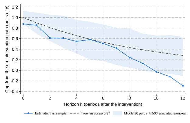
fig-sta01-one-draw.svg: Task 3’s estimates on the seed-2 sample (blue) against the true response 0.9^h (dashed) and the middle 90 percent of the 500 simulated samples (shaded). The estimate lies below the true response at every horizon, sits just under the band’s lower edge at h=0 (0.878940 against 0.879349), stays inside it from h=1 to h=10, and falls below it at h=11 and h=12. The band describes how the estimator varies across samples; it is not a confidence interval.
The caption the solution wrote, fig-sta01-one-draw-caption.txt:
Response of y to a one-unit intervention s_t, where one unit is one standard deviation because sigma_s = 1, estimated by local projections of y_(t+h) on a constant, s_t, and y_(t-1) in one simulated sample of T = 200 periods with rho = 0.9 (seed 2). The vertical axis is in units of y. Horizons are periods after the intervention; h = 0 is the period in which it occurs. The vertical axis measures the gap between the path with the intervention and the path without it, so zero means no different from that path, not y back where it started; the dashed line is the true response 0.9^h, and the band holds the middle 90 percent of estimates across 500 simulated samples (seed 3), which describes the estimator and is not a confidence interval.
Read the result. The Monte Carlo took 70.79 seconds for 500 samples at each \rho. At \rho=0.9 the mean estimate with the control lies below \theta_h at every horizon after impact, and from h=2 on the shortfall is more than twice its Monte Carlo standard error: −0.016848 against 0.006790 at h=2, and −0.048891 against 0.010044 at h=12. That is the small-sample bias Lecture 2 takes up, not a defect in the code: the row counts and both sets of summary values pass their checks. The control earns its place at impact, where the standard deviation across samples is 0.073358 with y_{t-1} and 0.217674 without it; by h=12 the two are 0.224580 and 0.241695, and at \rho=0.5 they start closer together (0.073010 and 0.094623) and converge sooner. The first 200 samples, which are what a student’s default run summarizes, give a mean of 0.370337 and a standard deviation of 0.211226 at \rho=0.9 and h=8, against 0.397256 and 0.228403 over all 500. The caption fills the four slots in order and ends by saying what the band is not.
Checks.
pass  Task 4: 199 - h rows with the control and 200 - h without
      value      0.37033659   target      0.37033700   |diff|  4.14e-07   tol  1.0e-06
pass  Task 4: with R = 200 the mean at rho = 0.9 and h = 8 is 0.370337
      value      0.21122564   target      0.21122600   |diff|  3.62e-07   tol  1.0e-06
pass  Task 4: with R = 200 the standard deviation at rho = 0.9 and h = 8 is 0.211226
pass  Task 4: without y_(t-1) the spread is larger at every h when rho = 0.9 (R = 200)
      value      0.39725582   target      0.39725600   |diff|  1.79e-07   tol  1.0e-06
pass  Task 4: with R = 500 the mean at rho = 0.9 and h = 8 is 0.397256
      value      0.22840343   target      0.22840300   |diff|  4.30e-07   tol  1.0e-06
pass  Task 4: with R = 500 the standard deviation at rho = 0.9 and h = 8 is 0.228403
pass  Task 4: the caption names the intervention and its unit
pass  Task 4: the caption gives the outcome's units
pass  Task 4: the caption gives the horizon unit
pass  Task 4: the caption names the counterfactual
pass  Task 4: the response graph is exported to output/pset/fig-sta01-one-draw.svg
Task 5 · Military news: the response, its variation, one episode
The last task leaves the simulation for Ramey and Zubairy’s quarterly data. The outcome is real GDP divided by trend GDP, and the news is divided by the previous quarter’s nominal trend GDP. Trend GDP is their series rgdp_pott6, which the authors call potential GDP and estimate as a sixth-degree polynomial trend in real GDP. get_rz.do found the workbook already verified in data/raw/, and import excel stores its columns as double.
*==========================================================================
* TASK 5 . Where the military-news coefficient's variation comes from
*          (Exercise 9; Lab 4)
*==========================================================================
do "data/raw/get_rz.do" "data/raw"
import excel using "data/raw/RZDAT.xlsx", sheet("rzdat") firstrow clear
drop if quarter < 1889
generate qdate = yq(1889, 1) + _n - 1
format qdate %tq
tsset qdate, quarterly
lp_assert "Task 5: 508 consecutive quarters, 1889Q1-2015Q4" : _N == 508 & abs(quarter - (1889 + (_n - 1)/4)) < 1e-6

generate double y     = rgdp/rgdp_pott6                  // real GDP / trend GDP
generate double newsy = news/(L.rgdp_pott6*L.pgdp)       // news / lagged nominal trend GDP
generate double g     = (ngov/pgdp)/rgdp_pott6           // real government spending / trend GDP
quietly count if newsy < .
local nnews = r(N)
lp_assert "Task 5: newsy has 504 nonmissing quarters" : `nnews' == 504
local k1950q3 = tq(1950q3) - tq(1889q1) + 1
lp_close newsy[`k1950q3'] 0.600073, tol(1e-6) label(Task 5: newsy in 1950Q3 is 0.600073)

tempname F
postfile `F' h double beta_h T_h using "output/pset/first_contact.dta", replace
forvalues h = 0/20 {
    quietly regress F`h'.y newsy L.y
    post `F' (`h') (_b[newsy]) (e(N))
}
postclose `F'

* shares of the variation in the h = 8 sample
quietly regress F8.y newsy L.y
local b8 = _b[newsy]
generate byte in8 = e(sample)
quietly summarize newsy if in8
generate double dev2 = (newsy - r(mean))^2 if in8
quietly summarize dev2
generate double share = dev2/r(sum)
preserve
keep if in8
gsort -share
generate double cumshare = sum(share)
keep in 1/10
generate rank = _n
keep rank qdate newsy share cumshare
format newsy share cumshare %9.6f
list rank qdate newsy share cumshare, clean noobs
lp_assert "Task 5: 1941Q4 has the largest share, 0.261211 (1e-6)" : qdate[1] == tq(1941q4) & abs(share[1] - 0.261211) < 1e-6
lp_assert "Task 5: 1950Q3 has the second largest share, 0.195838 (1e-6)" : qdate[2] == tq(1950q3) & abs(share[2] - 0.195838) < 1e-6
local share2 = cumshare[2]
local share6 = cumshare[6]
export delimited using "output/pset/sta01-news-shares.csv", replace datafmt
restore

* one episode out
quietly regress F8.y newsy L.y if qdate != tq(1950q3)
local b_drop = _b[newsy]
local n_drop = e(N)
lp_assert "Task 5: without 1950Q3 the h = 8 regression has 495 rows" : `n_drop' == 495
lp_close `b_drop' 0.433969, tol(1e-6) label(Task 5: at h = 8 without 1950Q3 the estimate is 0.433969)

* a source record: Ramey and Zubairy's controls at h = 10 (REP04 benchmark, irf_gdp_linear)
quietly regress F10.y newsy L(1/4).newsy L(1/4).y L(1/4).g
local b_rz10 = _b[newsy]
local n_rz10 = e(N)
lp_assert "Task 5: with Ramey-Zubairy controls the h = 10 regression has 490 rows" : `n_rz10' == 490
lp_close `b_rz10' 0.29376385, tol(1e-6) label(Task 5: with Ramey-Zubairy controls the h = 10 estimate is 0.29376385)

capture confirm file "handoff/l01-explorer-handoff.json"
if _rc == 0 {
    display as text _n "Lab 4 hypothesis in the Explorer record:"
    lp_json_get using "handoff/l01-explorer-handoff.json", key(lab4.hypothesis) display
    display as text "Stata: at h = 8 the estimate is " as result %8.6f `b8' as text " on the full sample and " ///
        as result %8.6f `b_drop' as text " on the `n_drop' rows without 1950Q3."
}

use "output/pset/first_contact.dta", clear
format beta_h %9.6f
list, clean noobs
lp_assert "Task 5: T_h = 504 - h" : T_h == 504 - h
lp_close beta_h[9] 0.361906, tol(1e-6) label(Task 5: beta_8 = 0.361906)
lp_close beta_h[11] 0.404210, tol(1e-6) label(Task 5: beta_10 = 0.404210)
quietly summarize beta_h
local gap_peak = abs(beta_h[11] - r(max))
lp_assert "Task 5: the response peaks at h = 10" : `gap_peak' < 1e-12
local b10 = beta_h[11]

local fc_intervention "Response to military-spending news worth one percent of the previous quarter's nominal trend GDP, from least squares of y_(t+h) on a constant, the news, and y_(t-1) over 1890Q1-2015Q4, with T_h = 504 - h rows (Ramey-Zubairy data, February 2018 package)."
local fc_outcome "The vertical axis is real GDP in percent of trend GDP, which is numerically beta_h per unit of the scaled news variable."
local fc_horizon "Horizons are quarters after the news arrives."
local fc_counterfactual "Read causally, the vertical axis is the gap between GDP and the path it would have followed without the news, a reading not yet argued; no bands are shown."

twoway (connected beta_h h, lcolor("`blue'") mcolor("`blue'") msymbol(O) msize(small) lwidth(medthick)), ///
       yline(0, lcolor("`rule'")) xlabel(0(2)20)                                     ///
       ylabel(0(0.1)0.5, format(%3.1f) angle(0) glcolor("`rule'"))                   ///
       xtitle("Quarters after the news arrives")                                      ///
       ytitle("Percent of trend GDP, per news worth 1 percent")                       ///
       legend(off) graphregion(color(white)) plotregion(color(white)) xsize(6.5) ysize(4)
graph export "output/pset/fig-sta01-first-contact.svg", replace
graph export "output/pset/fig-sta01-first-contact.png", replace width(1950)

local nya_units "The coefficients are responses of a level relative to a fitted trend per unit of scaled news, and whether that level, its change, or its accumulation answers the policymaker's question is not yet settled."
local nya_controls "One lag of GDP is a choice, and Ramey and Zubairy's controls lower the ten-quarter coefficient from `: display %5.3f `b10'' to `: display %5.3f `b_rz10''."
local nya_identification "Reading the curve as the effect of the news requires the news to be unpredictable and unrelated to the taxes, monetary policy, price controls, and wars that arrived with it, which nothing here has shown."
local nya_uncertainty "No standard error or band has been computed, and the overlapping horizons make the residuals serially correlated."
local nya_episodes "Two quarters, 1941Q4 and 1950Q3, supply `: display %4.1f 100*`share2'' percent of the variation in the news, and dropping 1950Q3 alone moves the eight-quarter estimate from `: display %5.3f `b8'' to `: display %5.3f `b_drop''."

tempname nf
file open `nf' using "output/pset/fig-sta01-first-contact-caption.txt", write text replace
file write `nf' `"`fc_intervention' `fc_outcome' `fc_horizon' `fc_counterfactual'"' _n
file close `nf'
file open `nf' using "output/pset/not-yet-argued.txt", write text replace
file write `nf' "What has not yet been argued" _n _n
foreach slot in units controls identification uncertainty episodes {
    file write `nf' `"`slot': `nya_`slot''"' _n
}
file close `nf'

foreach slot in intervention outcome horizon counterfactual {
    local len_`slot' = ustrlen(`"`fc_`slot''"')
}
lp_assert "Task 5: the caption names the intervention and its unit" : `len_intervention' >= 20
lp_assert "Task 5: the caption gives the outcome's units" : `len_outcome' >= 20
lp_assert "Task 5: the caption gives the horizon unit" : `len_horizon' >= 20
lp_assert "Task 5: the caption names the counterfactual" : `len_counterfactual' >= 20
foreach slot in units controls identification uncertainty episodes {
    local len = ustrlen(`"`nya_`slot''"')
    lp_assert "Task 5: the not-yet-argued paragraph has a sentence on `slot'" : `len' >= 40
}
capture confirm file "output/pset/fig-sta01-first-contact.svg"
local rc = _rc
lp_assert "Task 5: the response graph is exported to output/pset/fig-sta01-first-contact.svg" : `rc' == 0
Output.
Ramey-Zubairy data present in data/raw and verified (SHA-256).
...
. list rank qdate newsy share cumshare, clean noobs

    rank    qdate       newsy      share   cumshare
       1   1941q4    0.691893   0.261211   0.261211
       2   1950q3    0.600073   0.195838   0.457049
       3   1942q3    0.432791   0.100897   0.557946
       4   1950q4    0.402163   0.086893   0.644839
       5   1917q2    0.372915   0.074496   0.719335
       6   1941q2    0.340130   0.061734   0.781069
       7   1918q2    0.275022   0.039941   0.821010
       8   1940q2    0.259757   0.035515   0.856526
       9   1945q3   -0.219500   0.028682   0.885208
      10   1944q2   -0.196432   0.023145   0.908353
...
Lab 4 hypothesis in the Explorer record:
.     lp_json_get using "handoff/l01-explorer-handoff.json", key(lab4.hypothesis) display
Sample record. Dropping 1950Q3 will lower the h = 8 coefficient to about 0.30, because Korea is one of the two largest n
> ews quarters.
.     display as text "Stata: at h = 8 the estimate is " as result %8.6f `b8' as text " on the full sample and " ///
>         as result %8.6f `b_drop' as text " on the `n_drop' rows without 1950Q3."
Stata: at h = 8 the estimate is 0.361906 on the full sample and 0.433969 on the 495 rows without 1950Q3.
...
. list, clean noobs

     h     beta_h   T_h
     0   0.080313   504
     1   0.127363   503
     2   0.173289   502
     3   0.195597   501
     4   0.259141   500
     5   0.299480   499
     6   0.335977   498
     7   0.337931   497
     8   0.361906   496
     9   0.397627   495
    10   0.404210   494
    11   0.384037   493
    12   0.342677   492
    13   0.305247   491
    14   0.270833   490
    15   0.221056   489
    16   0.171908   488
    17   0.133997   487
    18   0.116266   486
    19   0.095899   485
    20   0.079552   484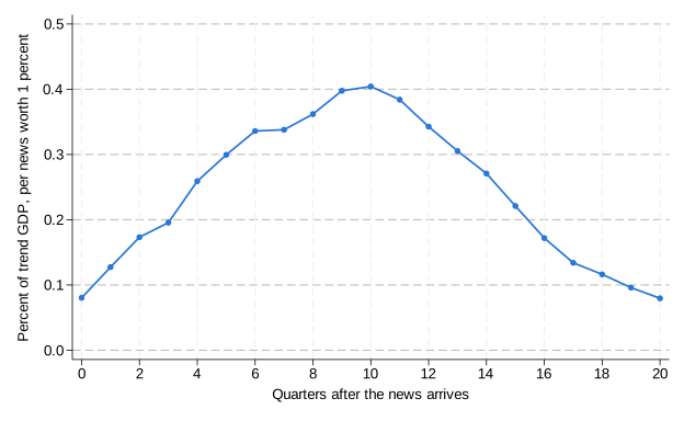
fig-sta01-first-contact.svg: the coefficient on the news in regressions of y_{t+h} on a constant, the news, and y_{t-1} over 1890Q1–2015Q4, with T_h=504-h rows, read as percent of trend GDP per news worth one percent of the previous quarter’s nominal trend GDP. The response rises from 0.080313 at impact to 0.404210 at h=10 and is back to 0.079552 at h=20. No bands are shown, and the causal reading is one of the things the accompanying paragraph lists as not yet argued.
The caption, fig-sta01-first-contact-caption.txt:
Response to military-spending news worth one percent of the previous quarter’s nominal trend GDP, from least squares of y_(t+h) on a constant, the news, and y_(t-1) over 1890Q1-2015Q4, with T_h = 504 - h rows (Ramey-Zubairy data, February 2018 package). The vertical axis is real GDP in percent of trend GDP, which is numerically beta_h per unit of the scaled news variable. Horizons are quarters after the news arrives. Read causally, the vertical axis is the gap between GDP and the path it would have followed without the news, a reading not yet argued; no bands are shown.
The written paragraph, not-yet-argued.txt:
What has not yet been argued

units: The coefficients are responses of a level relative to a fitted trend per unit of scaled news, and whether that level, its change, or its accumulation answers the policymaker's question is not yet settled.
controls: One lag of GDP is a choice, and Ramey and Zubairy's controls lower the ten-quarter coefficient from 0.404 to 0.294.
identification: Reading the curve as the effect of the news requires the news to be unpredictable and unrelated to the taxes, monetary policy, price controls, and wars that arrived with it, which nothing here has shown.
uncertainty: No standard error or band has been computed, and the overlapping horizons make the residuals serially correlated.
episodes: Two quarters, 1941Q4 and 1950Q3, supply 45.7 percent of the variation in the news, and dropping 1950Q3 alone moves the eight-quarter estimate from 0.362 to 0.434.
Read the result. The response rises from 0.080313 at impact to a peak of 0.404210 at h=10 and falls back to 0.079552 at h=20, on 504-h rows. In the regression’s own accounting, news worth one percent of the previous quarter’s nominal trend GDP goes with real GDP 0.40 percent of trend GDP higher ten quarters later; whether that is the effect of the news is what the paragraph says has not been argued. Two quarters, 1941Q4 and 1950Q3, supply 0.457049 of \sum_t(s_t-\bar s)^2 in the h=8 sample of 496 quarters, so the coefficient rests on two war episodes: dropping 1950Q3 alone raises the h=8 estimate from 0.361906 to 0.433969 on 495 rows, which refutes the sample record’s Lab 4 hypothesis of a fall to about 0.30. With Ramey and Zubairy’s own controls, four lags each of the news, y, and g, the h=10 coefficient is 0.29376385 on 490 rows, the linear GDP response in the course’s REP04 benchmark, so one lag of GDP is a choice that moves the peak by about a quarter. Each sentence of the paragraph takes its numbers from the run rather than from typing: 0.404 to 0.294, 45.7 percent, 0.362 to 0.434.
Checks.
pass  Task 5: 508 consecutive quarters, 1889Q1-2015Q4
pass  Task 5: newsy has 504 nonmissing quarters
      value      0.60007336   target      0.60007300   |diff|  3.64e-07   tol  1.0e-06
pass  Task 5: newsy in 1950Q3 is 0.600073
pass  Task 5: 1941Q4 has the largest share, 0.261211 (1e-6)
pass  Task 5: 1950Q3 has the second largest share, 0.195838 (1e-6)
pass  Task 5: without 1950Q3 the h = 8 regression has 495 rows
      value      0.43396908   target      0.43396900   |diff|  7.98e-08   tol  1.0e-06
pass  Task 5: at h = 8 without 1950Q3 the estimate is 0.433969
pass  Task 5: with Ramey-Zubairy controls the h = 10 regression has 490 rows
      value      0.29376385   target      0.29376385   |diff|  1.33e-09   tol  1.0e-06
pass  Task 5: with Ramey-Zubairy controls the h = 10 estimate is 0.29376385
pass  Task 5: T_h = 504 - h
      value      0.36190589   target      0.36190600   |diff|  1.14e-07   tol  1.0e-06
pass  Task 5: beta_8 = 0.361906
      value      0.40421035   target      0.40421000   |diff|  3.53e-07   tol  1.0e-06
pass  Task 5: beta_10 = 0.404210
pass  Task 5: the response peaks at h = 10
pass  Task 5: the caption names the intervention and its unit
pass  Task 5: the caption gives the outcome's units
pass  Task 5: the caption gives the horizon unit
pass  Task 5: the caption names the counterfactual
pass  Task 5: the not-yet-argued paragraph has a sentence on units
pass  Task 5: the not-yet-argued paragraph has a sentence on controls
pass  Task 5: the not-yet-argued paragraph has a sentence on identification
pass  Task 5: the not-yet-argued paragraph has a sentence on uncertainty
pass  Task 5: the not-yet-argued paragraph has a sentence on episodes
pass  Task 5: the response graph is exported to output/pset/fig-sta01-first-contact.svg
Grading notes
The machine checks confirm that each task’s numbers are right and that each written slot holds a sentence. What the sentences say is read by a person.
- Task 2. Omitting
if t >= 2from the regression without the control adds row 1, so the two regressions differ in rows as well as in the control; thesame_rowscheck catches it. - Task 4, the caption. One point per slot: the intervention and its unit, the outcome’s units, the horizon unit, and the counterfactual. Common mistakes: a vertical axis labeled “response of y” with nothing saying that zero means no different from the path without the intervention; calling the simulated band a confidence interval; omitting that one unit of s is one standard deviation.
- Task 5, the caption. The same four slots.
- Task 5, the paragraph. One point for each of the five sentences (units, controls, identification, uncertainty, dependence on a few episodes), and each sentence that cites a number must use the student’s own computed value.
- Task 5, common mistakes. Dividing the news by the same quarter’s nominal trend GDP instead of the previous quarter’s, which the 1950Q3 check (0.600073) catches; forcing T_h=503-h out of the row formula by dropping a quarter of data; reading the coefficient per unit of news rather than per 0.01; and treating the “not yet argued” paragraph as a defense of the estimate rather than a list of what is still missing.
3. The lab handoff, checked in Stata
The record checked is the sample shipped in the lab project, written by the Explorer’s own functions from its default data. Its Lab 2 and Lab 4 entries:
  "lab2": {
    "settings": {
      "h": 2,
      "control_y_lag": false,
      "single_episode": false
    },
    "file": "hand_table.csv",
    "rows": "2-10",
    "T_h": 9,
    "intervention_rows": [
      5,
      10
    ],
    "beta_h": 2.050024,
    "theta_h": 0.25,
    "used_in": "Exercise 4; STA01 Tasks 1-2",
    "prediction": "Sample record. Going from h = 0 to h = 2, rows 11 and 12 leave, and the intervention in row 12 leaves with them. The h = 2 slope will be no closer to 0.25 than the h = 0 slope is to 1."
  }
  ...
  "lab4": {
    "settings": {
      "h": 8,
      "controls": "toy",
      "rows": "drop1950q3"
    },
    "stored": {
      "beta_h": 0.433969,
      "T_h": 495,
      "beta_h_full_sample": 0.361906,
      "T_h_full_sample": 496
    },
    "hypothesis": "Sample record. Dropping 1950Q3 will lower the h = 8 coefficient to about 0.30, because Korea is one of the two largest news quarters.",
    "used_in": "Exercise 9; STA01 Task 5"
  }
handoff/check_handoff.do reran every computation the record reports: the Lab 2 regression on the hand table, all thirteen Lab 3 regressions on the draw, and the Lab 4 estimate from RZDAT.xlsx, together with its full-sample counterpart (handoff-check.csv). It reads those files exactly as the problem set does:
import delimited using "`hand'", clear      // handoff/hand_table.csv
import delimited using "`draw'", clear      // handoff/onedraw_rho09_seed2.csv
import excel using "data/raw/RZDAT.xlsx", sheet("rzdat") firstrow clear
import delimited stores the two CSV files’ columns as float and import excel stores the workbook’s as double, which is where the eighth decimals of the Stata column come from; the browser column is the record’s six-decimal number written out to eight places.
| Lab | Quantity | Browser | Stata | Difference | Result |
|---|---|---|---|---|---|
| Lab 2 | slope at h = 2 | 2.05002400 | 2.05002437 | 0.00000037 | agrees within 1e-6 |
| Lab 3 | slope at h = 0 | 0.87894000 | 0.87894028 | 0.00000028 | agrees within 1e-6 |
| Lab 3 | slope at h = 1 | 0.85326000 | 0.85326038 | 0.00000038 | agrees within 1e-6 |
| Lab 3 | slope at h = 2 | 0.61273700 | 0.61273705 | 0.00000005 | agrees within 1e-6 |
| Lab 3 | slope at h = 3 | 0.61104600 | 0.61104632 | 0.00000032 | agrees within 1e-6 |
| Lab 3 | slope at h = 4 | 0.54847700 | 0.54847739 | 0.00000039 | agrees within 1e-6 |
| Lab 3 | slope at h = 5 | 0.58309900 | 0.58309851 | −0.00000049 | agrees within 1e-6 |
| Lab 3 | slope at h = 6 | 0.50912000 | 0.50912038 | 0.00000038 | agrees within 1e-6 |
| Lab 3 | slope at h = 7 | 0.41778800 | 0.41778779 | −0.00000021 | agrees within 1e-6 |
| Lab 3 | slope at h = 8 | 0.24059500 | 0.24059456 | −0.00000044 | agrees within 1e-6 |
| Lab 3 | slope at h = 9 | 0.13029300 | 0.13029288 | −0.00000012 | agrees within 1e-6 |
| Lab 3 | slope at h = 10 | −0.02882100 | −0.02882139 | −0.00000039 | agrees within 1e-6 |
| Lab 3 | slope at h = 11 | −0.11720000 | −0.11719967 | 0.00000033 | agrees within 1e-6 |
| Lab 3 | slope at h = 12 | −0.29329700 | −0.29329663 | 0.00000037 | agrees within 1e-6 |
| Lab 4 | estimate at h = 8, drop1950q3 | 0.43396900 | 0.43396908 | 0.00000008 | agrees within 1e-6 |
| Lab 4 | estimate at h = 8, full sample | 0.36190600 | 0.36190589 | −0.00000011 | agrees within 1e-6 |
| Lab 4 | hypothesis: lower | 0.30000000 | 0.43396908 | 0.13396908 | direction refuted |
Every browser number was reproduced, the largest difference being 4.9e-7 (the browser rounds to six decimals and Stata’s draws are stored as float). The hypothesis is set against the estimate in handoff-check.log:
Hypothesis direction: lower.  Stata: the estimate moves from 0.361906 (496 rows) to 0.433969 (495 rows), so the rows rai
> se it.
.     display as text "Verdict: `verdict'."
Verdict: direction refuted.
.     local hyp_num = .
.     if "`num4'" != "" {
.         local hyp_num = `num4'
.         display as text "Hypothesized value " as result %8.4f `hyp_num' as text "; estimate " as result %8.6f `bsel' /
> //
>             as text "; miss " as result %8.4f abs(`bsel' - `hyp_num')
Hypothesized value   0.3000; estimate 0.433969; miss   0.1340
The record predicted that dropping 1950Q3 would lower the h=8 coefficient to about 0.30. Stata re-estimated 0.433969 on 495 rows, up from 0.361906 on 496, so the check records the direction as refuted and the value as missed by 0.134, as expectation 4 said it would. A refuted prediction is the result the lab is built to produce: the quarter with Korea’s news had pulled the slope down.
Discrepancy log
| Object | Published | Reproduced | Class | Diagnosis | Status |
|---|---|---|---|---|---|
| REP01 levels curve, h=0,\dots,10 | Figure 1a: 10,000 draws; the authors’ shipped means 0.99697095 to 0.42890212 | 500 draws: 1.00175746 to 0.43152008 | specification | Draw count reduced under D2; largest \lvert z\rvert against the 10,000-draw means 1.71, at h=2 | Accepted departure; labeled a statistical reproduction |
| REP01 means at 500 draws | Course benchmark, Stata/SE 18.5: 1.00175750 to 0.43152007 | StataNow/SE 19.5, rep01.do: 1.00175746 to 0.43152008 |
software | The authors average draws stored as float, rep01.do as double; the authors’ unchanged script in 19.5 returns the benchmark to every printed digit |
Resolved: largest difference 4\times10^{-8}, within 10^{-6}; no version difference (D1) |
| Draw 1 at h=0 | 1.06035137, the authors’ float storage |
1.06035143 | software | Rounding of r_level_0 to float (authors’ lines 125–128) |
Resolved: within 10^{-6} |
| Row counts T_h | Not stored; the benchmark derives 99-h from the construction | e(N) =99-h in every draw |
presentation | The authors keep coefficients only | Resolved: asserted in every draw |
| Sampling spread of the draws | Not available: the authors keep 11 draw rows and no standard errors | Standard deviation 0.105 to 0.397 and Monte Carlo standard error 0.0047 to 0.0178 across the build’s 500 draws | inference | The authors’ output discards the draws after averaging | Open for the published run; the build supplies its own from rep01-draws.dta |
Line 59, the term $a*l.d.y |
Present, with a set to 0.00 on line 57 |
Omitted | specification | A zero coefficient; the unchanged script and rep01.do agree at every horizon |
Resolved: within 4\times10^{-8} |
| Lines 5–7 and 13, working folder and font | cap cd to the authors’ Dropbox folders; graph set window fontface "Palatino" |
No effect in batch; the authors’ PDF is written to output/rep01-author/ |
presentation | Paths that do not exist fail silently; batch mode has no graph window | Accepted; on 2026-09-14 the two cap cd lines were commented out in the shipped copy so that the archive holds no absolute path, and vendor/jel-code/SOURCE.md records both hashes |
| Figure 1a’s other curves | Long-difference, cumulative-difference, and AR(1) curves drawn with the levels curve | Not reproduced | specification | Outside REP01’s target | Deferred to REP02 (Practicum 02) |
| Ramey–Zubairy data for Task 5 | RZDAT.xlsx, February 2018 package, SHA-256 b2d85087…8c6120 |
The same file, verified before use | data | No redistribution license in the package: fetched by get_rz.do rather than shipped (D5, D35) |
Resolved; the automatic download worked on 2026-09-13 |
| The Explorer’s draw file | 0.678-style numbers written by the browser |
.678-style numbers written by Stata; SHA-256 differs, values identical |
presentation | JavaScript and Stata format numbers differently | Resolved: the problem set and the handoff check compare values, not bytes |
The lab project departs from the practicum plan in layout only. The plan named five scripts under code/ and PDF figures; the project follows the course’s practicum layout (replication/, starter/, solution/, tests/, handoff/) and exports SVG and PNG figures for the web. The plan’s REP01 steps are rep01.do, and its five STA01 tasks, with their assertions, are starter/pset.do.